Andrew NG deep learning--chapter 1& chapter 2
標簽: python deeplearning machinelearning
import numpy as np
from lr_utils import load_dataset
#we only use these two modules currently
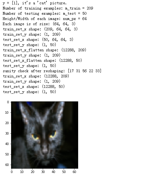
train_set_x_orig, train_set_y_orig, test_set_x_orig, test_set_y_orig, classes = load_dataset()
m_train = train_set_x_orig.shape[0] #209 pic(train set)m_test = test_set_x_orig.shape[0] #50 pic(test set)
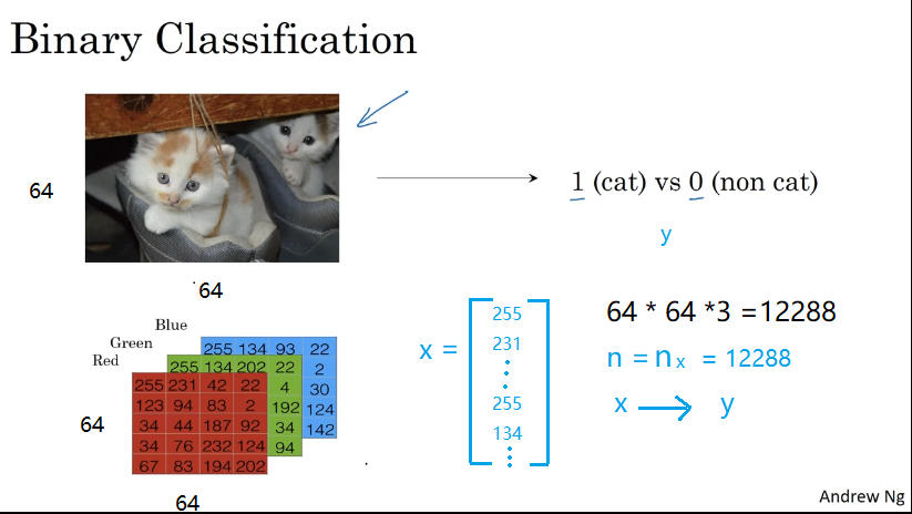
num_px = train_set_x_orig.shape[1] #64 px
train_set_x_flatten = train_set_x_orig.reshape(m_train, num_px * num_px * 3).T test_set_x_flatten = test_set_x_orig.reshape(m_test, num_px * num_px * train_set_x_orig.shape[3]).T #209*64*64*3 train set /50*64*64*3 test set 12288*209 12288*50 train_set_x = train_set_x_flatten / 255 #標準化操作 divide each pix by 255
test_set_x = test_set_x_flatten / 255A、sigmoid(x)函數(upforward propagation )
A=σ(wTX+b)=(a(0),a(1),...,a(m?1),a(m))
def sigmoid(x):
    s = 1.0 / (1 + 1 / np.exp(x))
    return s
B、initialize w&b
def initializewithzeros(dim):
    w = np.zeros((dim, 1))
    b = 0
    # we have to transfrom w in the following step, thus we initialize it as dim*1
    assert (w.shape == (dim, 1))
    assert (isinstance(b, float) or isinstance(b, int))

    return w, b
# X equals to 12288*209 thus when we calculate the wTX+b, we have to do matrix transpose for w.(from 12288*1 to 1*12288) w.T*X+b is 1*209
C、 propagate(forward, Cost calculation, backward gradient)
def propagate(w, b, X, Y):
    A = sigmoid(np.dot(w.T, X)+b)
    # shape of A: 1*209
    m = X.shape[1] #209
    cost = -(1.0 / m) * np.sum(Y * np.log(A) + (1 - Y) * np.log(1 - A))
#compared with train_set_y

    dw = (1.0/m)* np.dot(X, (A - Y).T)
    # shape of dw: [64*64*3 1]
    db = 1.0 / m * np.sum(A - Y, axis=1, keepdims=True)
    cost = np.squeeze(cost)
    assert (cost.shape == ())
    assert (dw.shape == w.shape)
    assert (db.dtype == float)

    grads = {"dw": dw,
             "db": db
             }

    return grads, cost
calculate cost function:
J=?1m∑mi=1y(i)log(a(i))+(1?y(i))log(1?a(i))
J=?1m∑mi=1y(i)log(a(i))+(1?y(i))log(1?a(i))J=?1m∑i=1my(i)log?(a(i))+(1?y(i))log?(1?a(i))
calculate backward gradient:
D, using dw,db to update w&b
def optimize(w, b, X, Y, num_iterations, learning_rate, print_cost=True):
    costs = []


    for i in range(num_iterations):
        grads, cost = propagate(w, b, X, Y)

        dw = grads["dw"]
        db = grads["db"]
        if i % 100 == 0:
            costs.append(cost)
        w = w - dw * learning_rate
        b = b - db * learning_rate

        if print_cost and i % 100 == 0:
            print("Cost after iteration %i:%f" % (i, cost))

        params = {"w": w,
                  "b": b}
        grads = {"dw": dw,
                 "db": db
                 }

    return params, grads, costs
w and b update step by step thus the w and b will be more accurate, the output will be coincided with the model(iteration time)
E, Prediction (get the output y_prediction)
def predict(w, b, X):
    m = X.shape[1]
    y_prediction = np.zeros((1, m))
#    w = w.reshape(X.shape[0], 1)
    A = sigmoid(np.dot(w.T, X) + b)
    for i in range(A.shape[1]):
        y_prediction = np.floor(A + 0.5)

    assert (y_prediction.shape == (1, m))

    return y_prediction
m equals to 209, then we set an blank matrix(y_prediction) to save the data.
w equals to 12288*1 not necessary here!
A equals to 1*209, it proves the output of(y/n) every pic.
F , merge into the model function
def model(X_train, Y_train, X_test, Y_test, num_iterations=2000, learning_rate=0.5, print_cost=False):
    w, b = initializewithzeros(X_train.shape[0])
    parameters, gradients, costs = optimize(w, b, X_train, Y_train, num_iterations, learning_rate, print_cost)

    w = parameters['w']
    b = parameters['b']

    Y_prediction_train = predict(w, b, X_train)
    Y_prediction_test = predict(w, b, X_test)

    print("train accuracy:{} %".format(100 - np.mean(np.abs(Y_prediction_train - Y_train)) * 100))

    print("test accuracy:{} %".format(100 - np.mean(np.abs(Y_prediction_test - Y_test)) * 100))

    d = {"costs": costs,
         "Y_prediction_test": Y_prediction_test,
         "Y_prediction_train": Y_prediction_train,
         "w": w,
         "b": b,
         "learning_rate": learning_rate,
         "num_iterations": num_iterations}

    return d
get the prediction by using the predict function
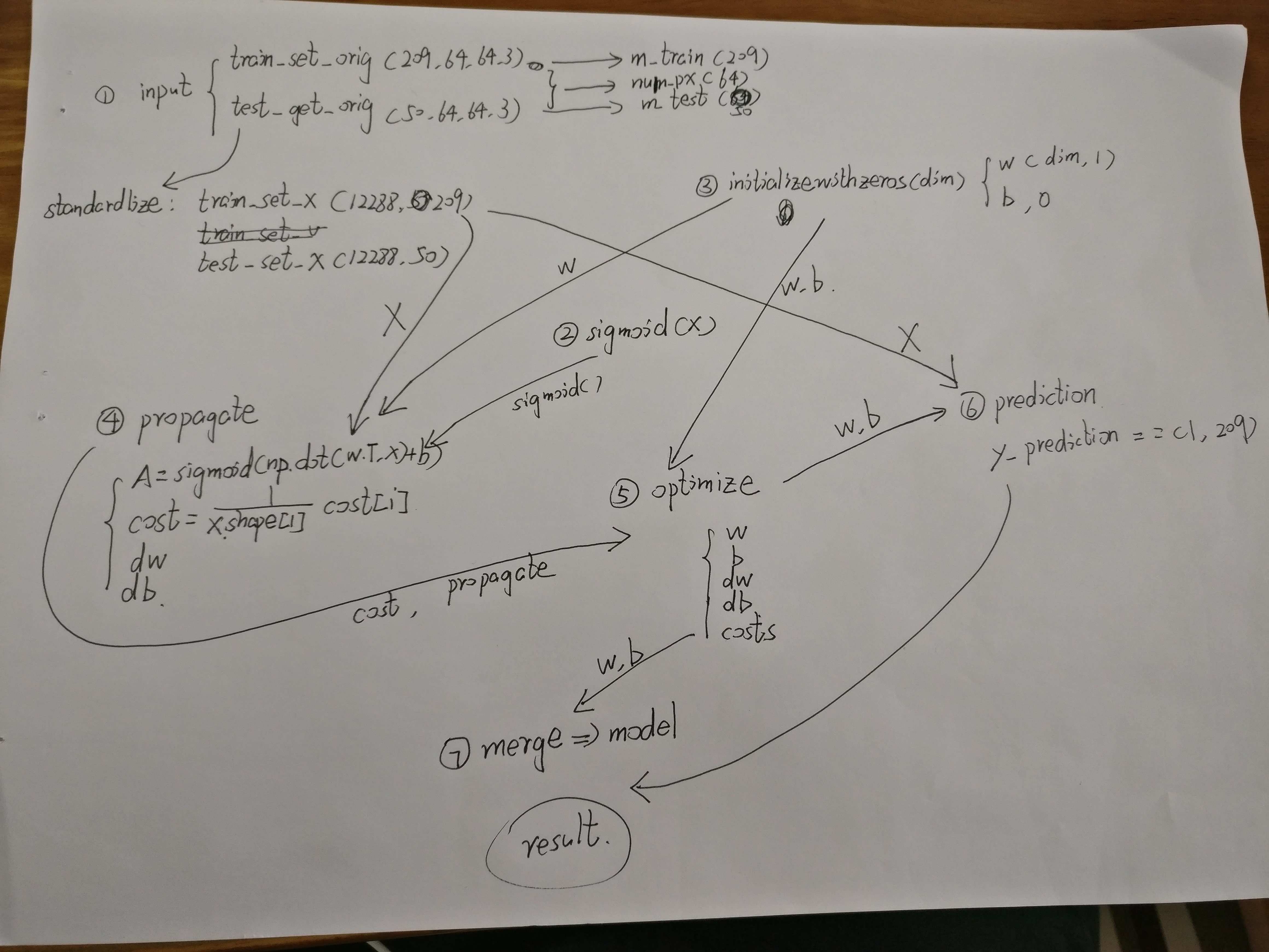
later on , I will also attach the mindnode pic for chapter 1 and 2, which is very useful for us to illustrate the total flow.
智能推薦

Machine Learning(Andrew Ng)ex1.linear regression
Linear Regression Population Profit 0 6.1101 17.5920 1 5.5277 9.1302 2 8.5186 13.6620 3 7.0032 11.8540 4 5.8598 6.8233 Ones Population 0 1 6.1101 1 1 5.5277 2 1 8.5186 3 1 7.0032 4 1 5.8598 Profit 0 1...
Andrew NG 機器學習 練習1-Linear Regression
在本次練習中,需要實現一個單變量的線性回歸。假設有一組歷史數據<城市人口,開店利潤>,現需要預測在哪個城市中開店利潤比較好? 歷史數據如下:第一列表示城市人口數,單位為萬人;第二列表示利潤,單位為10,000$ ex1data1.txt 6.1101,17.592 5.5277,9.1302 8.5186,13.662 7.0032,11.854 … … 用...
deep learning Andrew學習筆記
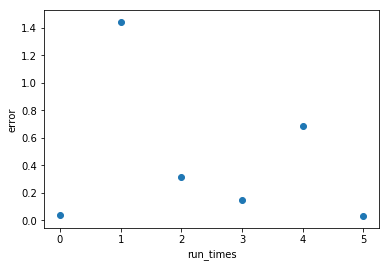
Freezing one weight cause the same result with unfreezing(Deep learning書的一個練習) 在神經網絡訓啦中,凍結某權重,總的誤差依然會降為0的現象。 看到這兩次輸出的weight結果差別不大,說明第三個weight確實不怎么影響結果,換個weight試試,還是error還是降低到了0……,控制兩個呢 控...
Andrew Ng 深度學習課后測試記錄-01-week2-答案
代碼標注及運行、調試結果 tips:深度學習中的很多錯誤軟件來自矩陣/向量的維度不匹配,要注意檢查 1.準備工作 結果: 2.數組訪問技巧 3.學習算法的一般體系結構 設計一種簡單的算法來區分貓圖像和非貓圖像。 您將使用神經網絡思維模式構建Logistic回歸。 下圖解釋了為什么Logistic回歸實際上是一個非常簡單的神經網絡! 數學表達式: 針對樣例 cost函數: ...
Coursera | Andrew Ng (01-week2)—神經網絡基礎
在吳恩達深度學習視頻以及大樹先生的博客提煉筆記基礎上添加個人理解,原大樹先生博客可查看該鏈接地址大樹先生的博客- ZJ Coursera 課程 |deeplearning.ai |網易云課堂 CSDN:http://blog.csdn.net/junjun_zhao/article/details/79226016 第二周 神經網絡基礎 (Basics of Neural Network Prog...
猜你喜歡
Coursera | Andrew Ng (01-week-2-2.13)—向量化 Logistic 回歸
該系列僅在原課程基礎上部分知識點添加個人學習筆記,或相關推導補充等。如有錯誤,還請批評指教。在學習了 Andrew Ng 課程的基礎上,為了更方便的查閱復習,將其整理成文字。因本人一直在學習英語,所以該系列以英文為主,同時也建議讀者以英文為主,中文輔助,以便后期進階時,為學習相關領域的學術論文做鋪墊。- ZJ Coursera 課程 |deeplearning.ai |網易云課堂 轉載請注明作者和...


freemarker + ItextRender 根據模板生成PDF文件
1. 制作模板 2. 獲取模板,并將所獲取的數據加載生成html文件 2. 生成PDF文件 其中由兩個地方需要注意,都是關于獲取文件路徑的問題,由于項目部署的時候是打包成jar包形式,所以在開發過程中時直接安照傳統的獲取方法沒有一點文件,但是當打包后部署,總是出錯。于是參考網上文章,先將文件讀出來到項目的臨時目錄下,然后再按正常方式加載該臨時文件; 還有一個問題至今沒有解決,就是關于生成PDF文件...
電腦空間不夠了?教你一個小秒招快速清理 Docker 占用的磁盤空間!
Docker 很占用空間,每當我們運行容器、拉取鏡像、部署應用、構建自己的鏡像時,我們的磁盤空間會被大量占用。 如果你也被這個問題所困擾,咱們就一起看一下 Docker 是如何使用磁盤空間的,以及如何回收。 docker 占用的空間可以通過下面的命令查看: TYPE 列出了docker 使用磁盤的 4 種類型: Images:所有鏡像占用的空間,包括拉取下來的鏡像,和本地構建的。 Con...

requests實現全自動PPT模板
http://www.1ppt.com/moban/ 可以免費的下載PPT模板,當然如果要人工一個個下,還是挺麻煩的,我們可以利用requests輕松下載 訪問這個主頁,我們可以看到下面的樣式 點每一個PPT模板的圖片,我們可以進入到詳細的信息頁面,翻到下面,我們可以看到對應的下載地址 點擊這個下載的按鈕,我們便可以下載對應的PPT壓縮包 那我們就開始做吧 首先,查看網頁的源代碼,我們可以看到每一...