Andrew Ng 深度學習課程Deeplearning.ai 編程作業——deep Neural network for image classification(1-4.2)
1.Package
import numpy as np #scientific compute package
import matplotlib.pyplot as plt #graphs package
import h5py #contact with h5 file
import scipy
from scipy import ndimage #import our image and reshape to the specific size
from A_deeper_neural_network import initialize_parameters_deep,linear_activation_forward,compute_cost,linear_activation_backward
from A_deeper_neural_network import update_parameters #這里我導入了自己寫的文件的模塊A_deeper_neural_network
plt.rcParams["figure.figsize"]=(5.0,4.0) #set the figure figzie to (5.0,4.0)
plt.rcParams["image.interpolation"]="nearest"
plt.rcParams["image.cmap"]='gray'
np.random.seed(1) #set the random initial seed
def load_dataset(): #定義導入文件的函數
train_dataset=h5py.File ('/home/hansry/python/DL/1-4/assignment4/datasets/train_catvnoncat.h5',"r")
train_set_x_orig = np.array(train_dataset["train_set_x"][:])
train_set_y_orig = np.array(train_dataset["train_set_y"][:])
test_dataset=h5py.File('/home/hansry/python/DL/1-4/assignment4/datasets/test_catvnoncat.h5',"r")
test_set_x_orig = np.array(test_dataset["test_set_x"][:])
test_set_y_orig = np.array(test_dataset["test_set_y"][:])
classes = np.array(test_dataset["list_classes"][:]) # the list of classes
train_set_y_orig=train_set_y_orig.reshape((1,train_set_y_orig.shape[0]))
test_set_y_orig=test_set_y_orig.reshape(1,test_set_y_orig.shape[0])
return train_set_x_orig,train_set_y_orig,test_set_x_orig,test_set_y_orig,classes
train_set_x_orig,train_set_y,test_set_x_orig,test_set_y,classes=load_dataset()
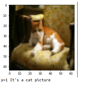
index=7
plt.imshow(train_set_x_orig[index]) #to show the package
plt.show()
print("y="+str(train_set_y[0][index])+" It's a "+classes[train_set_y[0][index]].decode("utf-8")+" picture")
Expected output:
2.datasets
train_set_x_orig,train_set_y,test_set_x_orig,test_set_y,classes=load_dataset()
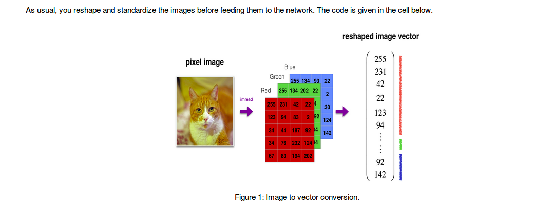
num_px=train_set_x_orig.shape[1]
train_x_flatten=train_set_x_orig.reshape(train_set_x_orig.shape[0],num_px*num_px*3).T
test_x_flatten=test_set_x_orig.reshape(test_set_x_orig.shape[0],num_px*num_px*3).T
train_x=train_x_flatten/255 #centralize and normorlize the datasets
test_x=test_x_flatten/255
print ("train_x's shape:"+str(train_x.shape))
print ("test_x's shape:"+str(test_x.shape))
Expected output:
train_x's shape:(12288, 209)
test_x's shape:(12288, 50)
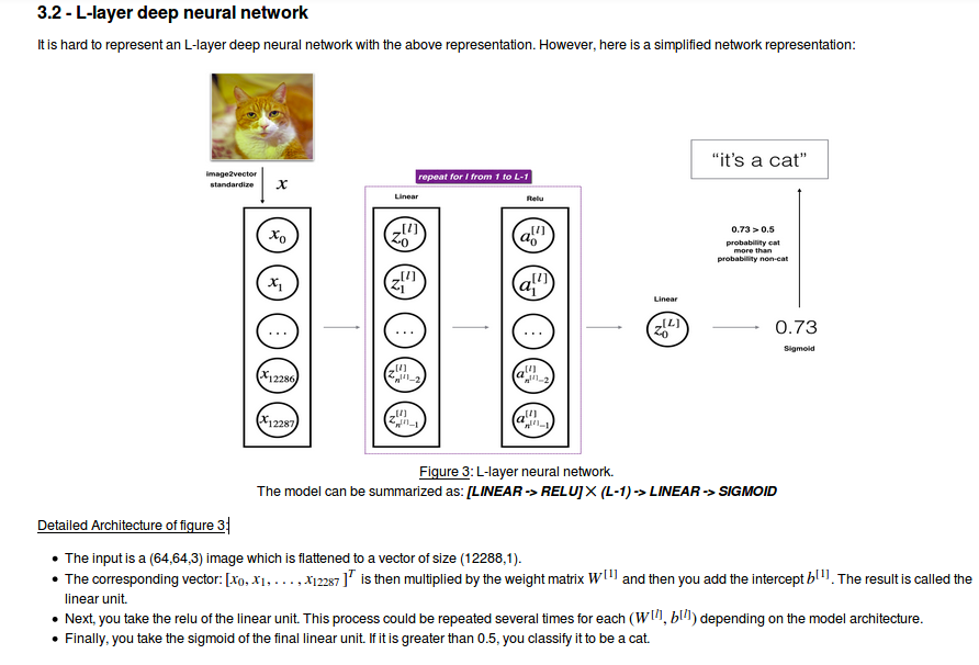
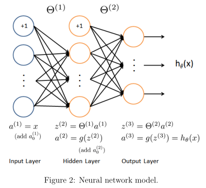
##3.Architecture of your model ##
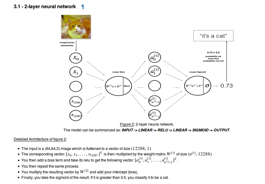
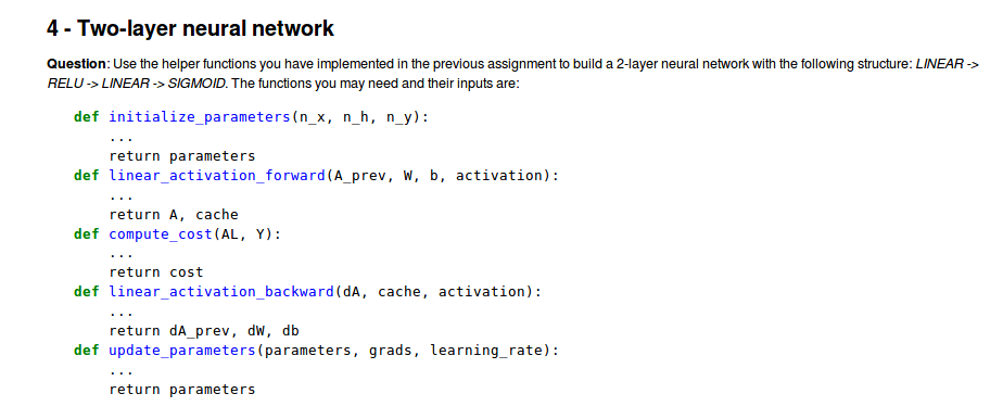
4.Two-layer neural network
n_x=12288
n_h=7
n_y=1
layer_dims=(n_x,n_h,n_y)
def two_layer_model(X,Y,layers_dims,learning_rate,num_iterations,print_cost=True):
np.random.seed(1)
parameters=initialize_parameters_deep(layer_dims)
costs=[]
grads={}
W1=parameters["W1"]
b1=parameters["b1"]
W2=parameters["W2"]
b2=parameters["b2"]
for i in range(num_iterations):
A1,cache1=linear_activation_forward(X,W1,b1,activation="relu")
# print cache1[0][0].shape
# print A1
A2,cache2=linear_activation_forward(A1,W2,b2,activation="sigmoid")
cost=compute_cost(A2,Y)
# costs.append(cost)
dA2=-(np.divide(Y,A2)-np.divide(1-Y,1-A2))
dA1,dW2,db2=linear_activation_backward(dA2,cache2,activation="sigmoid")
dA0,dW1,db1=linear_activation_backward(dA1,cache1,activation="relu")
grads["dW2"]=dW2
grads["db2"]=db2
grads["dW1"]=dW1
grads["db1"]=db1
parameters=update_parameters(parameters,grads,learning_rate)
W1=parameters["W1"]
b1=parameters["b1"]
W2=parameters["W2"]
b2=parameters["b2"]
if print_cost and i%100==0:
print ("cost after iteration{}:{}".format(i,np.squeeze(cost)))
if i%100==0:
costs.append(cost)
costs=np.squeeze(costs)
plt.plot(costs)
plt.ylabel("cost")
plt.xlabel("iterations per one thousand")
plt.title("learning rate :"+str(learning_rate))
plt.show()
return parameters
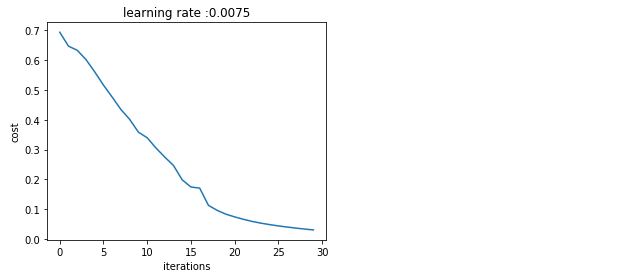
parameters=two_layer_model(train_x,train_set_y,layer_dims,learning_rate=0.0075,num_iterations=3000,print_cost=True)
Expected output:
cost after iteration0:0.69304973566
cost after iteration100:0.646432095343
cost after iteration200:0.632514064791
cost after iteration300:0.601502492035
cost after iteration400:0.560196631161
cost after iteration500:0.515830477276
cost after iteration600:0.475490131394
cost after iteration700:0.433916315123
cost after iteration800:0.40079775362
cost after iteration900:0.358070501132
cost after iteration1000:0.339428153837
cost after iteration1100:0.30527536362
cost after iteration1200:0.274913772821
cost after iteration1300:0.246817682106
cost after iteration1400:0.198507350375
cost after iteration1500:0.174483181126
cost after iteration1600:0.170807629781
cost after iteration1700:0.113065245622
cost after iteration1800:0.0962942684594
cost after iteration1900:0.0834261795973
cost after iteration2000:0.0743907870432
cost after iteration2100:0.0663074813227
cost after iteration2200:0.0591932950104
cost after iteration2300:0.0533614034856
cost after iteration2400:0.0485547856288
cost after iteration2500:0.0441405969255
cost after iteration2600:0.0403456450042
cost after iteration2700:0.0368412198948
cost after iteration2800:0.0336603989271
cost after iteration2900:0.0307555969578
def prediction(parameters,X,Y):  #對訓練集和預測集進行精度評判
    W1=parameters["W1"]
    b1=parameters["b1"]
    W2=parameters["W2"]
    b2=parameters["b2"]
    A1,cache1=linear_activation_forward(X,W1,b1,activation="relu")
    A2,cache2=linear_activation_forward(A1,W2,b2,activation="sigmoid")
    predictions=(A2>0.5)  #將大于0的設置為1
    accuracy_per=float(np.dot(Y,predictions.T)+np.dot(1-Y,1-predictions.T))/float(Y.size)*100
    return predictions,accuracy_per

predictions,accuracy=prediction(parameters,train_x,train_set_y)
print ("train_accuracy: "+str(accuracy))

predictions,accuracy=prediction(parameters,test_x,test_set_y)
print ("test_accuracy: "+str(accuracy))
Expected output:
train_accuracy: 100.0
test_accuracy: 72.0
Congratulations! It seems that your 2-layer neural network has better performance (72%) than the logistic regression implementation (70%, assignment week 2). Let’s see if you can do even better with an LL-layer model.
5.L-layer Neural Network
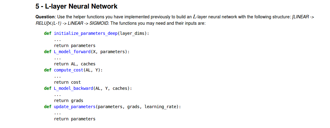
layer_dims=[12288,20,7,5,1]
def L_layer_model(X,Y,layer_dims,num_iterations,learning_rate,print_cost):
np.random.seed(1)
parameters=initialize_parameters_deep(layer_dims)
costs=[]
for i in range(num_iterations):
AL,caches=L_model_layer(X,parameters)
cost_L_model=compute_cost(AL,Y)
grads=L_model_backward(AL,Y,caches)
parameter=update_parameters(parameters,grads,learning_rate)
if print_cost and i%100==0:
print ("cost after iterations{}:{}".format(i,cost_L_model))
if i%100==0:
costs.append(cost_L_model)
return parameter,costs
def prediction_L_model(parameters,X,Y):
AL,caches=L_model_layer(X,parameters)
predictions=(AL>0.5)
accuracy=float(np.dot(Y,predictions.T)+np.dot(1-Y,(1-predictions).T))/float(Y.size)*100
return accuracy,predictions
parameters,costs=L_layer_model(train_x,train_set_y,layer_dims,learning_rate=0.01,num_iterations=3000,print_cost=True)
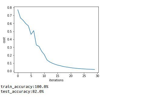
costs=np.squeeze(costs)
plt.plot(costs)
plt.ylabel("cost")
plt.xlabel("iterations")
plt.show()
train_accuracy,train_predictions=prediction_L_model(parameters,train_x,train_set_y)
print ("train_accuracy:"+str(train_accuracy)+"%")
test_accuracy,test_predictions=prediction_L_model(parameters,test_x,test_set_y)
print ("test_accuracy:"+str(test_accuracy)+"%")
Expected output:
train_x's shape:(12288, 209)
test_x's shape:(12288, 50)
cost after iterations0:0.771749328424
cost after iterations100:0.669269663073
cost after iterations200:0.638873866746
cost after iterations300:0.597884241863
cost after iterations400:0.568827182668
cost after iterations500:0.461260004201
cost after iterations600:0.508483601988
cost after iterations700:0.32759554358
cost after iterations800:0.31039799625
cost after iterations900:0.24883052978
cost after iterations1000:0.207309305492
cost after iterations1100:0.140485374517
cost after iterations1200:0.115670324218
cost after iterations1300:0.0992596314732
cost after iterations1400:0.0858446278017
cost after iterations1500:0.0749750709344
cost after iterations1600:0.0678088205921
cost after iterations1700:0.0584015277879
cost after iterations1800:0.0520540925361
cost after iterations1900:0.0476796512902
cost after iterations2000:0.0422589466752
cost after iterations2100:0.0377972361751
cost after iterations2200:0.0347303021461
cost after iterations2300:0.0313911132159
cost after iterations2400:0.0287875716657
cost after iterations2500:0.0264843633988
cost after iterations2600:0.0243811278867
cost after iterations2700:0.0226565055434
cost after iterations2800:0.021282864075
cost after iterations2900:0.0196948174932
在這里需要注意的是初始化權重的函數,即 initialize_parameters_deep(layer_dims),具體內容如下:
def initialize_parameters_deep(layer_dims):
    """
    Arguments:
    layer_dims -- python array (list) containing the dimensions of each layer in our network

    Returns:
    parameters -- python dictionary containing your parameters "W1", "b1", ..., "WL", "bL":
                    Wl -- weight matrix of shape (layer_dims[l], layer_dims[l-1])
                    bl -- bias vector of shape (layer_dims[l], 1)
    """

    np.random.seed(1)
    parameters = {}
    L = len(layer_dims)            # number of layers in the network

    for l in range(1, L):
        parameters['W' + str(l)] = np.random.randn(layer_dims[l], layer_dims[l-1]) / np.sqrt(layer_dims[l-1]) #*0.01,注意這里不是乘以0.01,因為會陷入局部極小值
        parameters['b' + str(l)] = np.zeros((layer_dims[l], 1))

        assert(parameters['W' + str(l)].shape == (layer_dims[l], layer_dims[l-1]))
        assert(parameters['b' + str(l)].shape == (layer_dims[l], 1))


    return parameters
6.Result Analysis
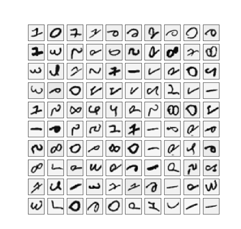
First, let’s take a look at some images the L-layer model labeled incorrectly. This will show a few mislabeled images.
def mislabeled_images(classes,X,Y,p):
    precision=Y+p
    print precision
    mislabel_indices=np.asarray(np.where(precision==1))
    print mislabel_indices
    num_image=mislabel_indices.shape[1]
    plt.rcParams["figure.figsize"]=(10.0,10.0)
    for i in range(num_image):
        index=mislabel_indices[1,i]
        plt.subplot(num_image//3,3,i+1)
        plt.imshow(X[:,index].reshape(64,64,3),interpolation='nearest')
        plt.axis=('off')
        plt.title("Prediction:"+str(classes[int(p[0,index])].decode("utf-8"))+"\n"+"Real:"+str(classes[Y[0,index]].decode("utf-8")))


mislabeled_images(classes,test_x,test_set_y,test_predictions)
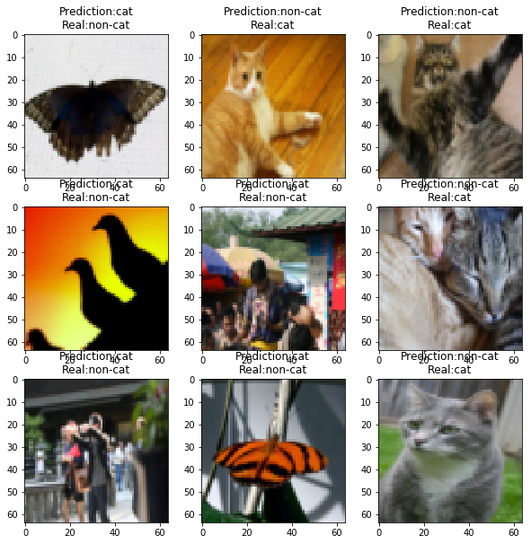
如上圖所示,在50張圖中,9張預測錯誤,準確率為82%
A few type of images the model tends to do poorly on include:
Cat body in an unusual position
Cat appears against a background of a similar color
Unusual cat color and species
Camera Angle
Brightness of the picture
Scale variation (cat is very large or small in image)
智能推薦
Andrew NG 機器學習 練習4-Neural Networks Learning
Introduction 我們將實現神經網絡的反向傳播算法,并將其應用到手寫數字識別中。 1 神經網絡 在以前的練習中,我們實現了 神經網絡的前饋傳播,并用我們提供的權重值,將其應用到了預測手寫字體的任務中。在這個練習中,你講實現后向傳播算法來學習神經網絡的參數。 1.1 可視化數據 每個訓練樣例,是一個20*20像素的圖片灰度數值。每個像素通過一個浮點類型的值來表示灰度值。20*20像素的數值被...
Andrew Ng Machine Learning——Work(Four)——Feedback neural network(Based on Python 3.7)
所用數據集鏈接:反向傳播網絡所用數據集(ex4data1.mat,ex4weights.mat),提取碼:c3yy 目錄 Feedback neural network 1.0 Package 1.1 Load data 1.2 Visualization data 1.3 Data preprocess 1.4 Load weights 1.5 Unrolling data 1.6 Deseri...
吳恩達(Andrew Ng)deep learning課程-Sequence Models編程作業Emojify Pycharm實現
本作業所有資料均來自吳恩達在Coursera課程平臺,深度學習專項課程第五門Sequence Models課程中第二周的課后作業Emogify。 課程鏈接為:https://www.coursera.org/learn/nlp-sequence-models 本節作業所需資料以及代碼可從該作業文件目錄下下載,鏈接為: https://www.coursera.org/learn/nlp-seque...
Coursera深度學習課程 DeepLearning.ai 編程作業——Improvise a Jazz Solo with an LSTM Network
Improvise a Jazz Solo with an LSTM Network ? Welcome to your final programming assignment of this week! In this notebook, you will implement a model that uses an LSTM to generate music. You will even ...
Andrew NG機器學習線性回歸編程作業
備注: Coursera上Andrew Ng的機器學習課程有8次編程作業。本帖記錄我練習過程中學到的知識,希望對大家有幫助。Andrew NG機器學習線性回歸編程作業詳細分析,這篇耗費巨大心血,非常適合小白去做NG課程作業時參考,部分代碼不好理解(先放棄),重點理解NG留的那些空的代碼,然后參考我整理的另一篇博客,線性規劃的Matlab代碼總結,結合著看,慢慢就懂了,加油 背景 在本次練習中,需要...
猜你喜歡
Andrew NG機器學習邏輯回歸編程作業
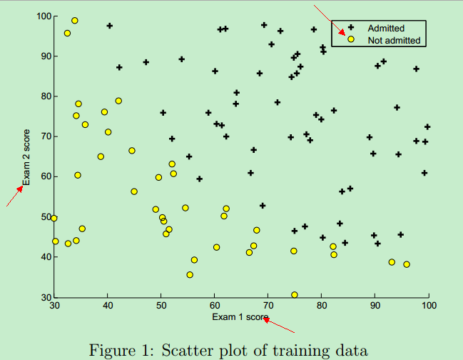
Exercise 2:Logistic Regression—實現一個邏輯回歸 問題描述:用邏輯回歸根據學生的考試成績來判斷該學生是否可以入學。 這里的訓練數據(training instance)是學生的兩次考試成績,以及TA是否能夠入學的決定(y=0表示成績不合格,不予錄取;y=1表示錄取) 因此,需要根據trainging set 訓練出一個classification mode...
Andrew Ng-Convolutional Neural Networks 第二周作業 Keras Tutorial
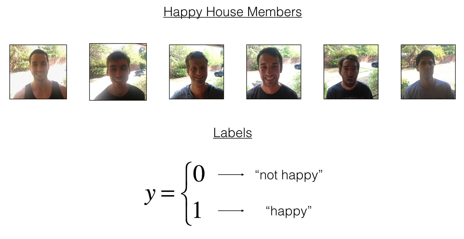
233卷積網絡的全自動化 就是給出了一些基本的代碼示例,然后就讓你放飛自我了(Feel free to use the suggested outline in the text above to get started, and run through the whole) 題目是給出了一堆人臉,然后判斷他們是否開心 基本信息就這些,接下來就放飛自我,那就很簡單了。。。隨便就能實現一個簡單的VG...


freemarker + ItextRender 根據模板生成PDF文件
1. 制作模板 2. 獲取模板,并將所獲取的數據加載生成html文件 2. 生成PDF文件 其中由兩個地方需要注意,都是關于獲取文件路徑的問題,由于項目部署的時候是打包成jar包形式,所以在開發過程中時直接安照傳統的獲取方法沒有一點文件,但是當打包后部署,總是出錯。于是參考網上文章,先將文件讀出來到項目的臨時目錄下,然后再按正常方式加載該臨時文件; 還有一個問題至今沒有解決,就是關于生成PDF文件...
電腦空間不夠了?教你一個小秒招快速清理 Docker 占用的磁盤空間!
Docker 很占用空間,每當我們運行容器、拉取鏡像、部署應用、構建自己的鏡像時,我們的磁盤空間會被大量占用。 如果你也被這個問題所困擾,咱們就一起看一下 Docker 是如何使用磁盤空間的,以及如何回收。 docker 占用的空間可以通過下面的命令查看: TYPE 列出了docker 使用磁盤的 4 種類型: Images:所有鏡像占用的空間,包括拉取下來的鏡像,和本地構建的。 Con...