pytorch學習筆記(四)
pytorch學習筆記(四)
1.前言
前面我們已經簡單建立一個分類器的神經網絡,雖然訓練的效果比較一般,不過這就是一個神經網絡大體應該具備的特征,后面的優化也就是基于這個不斷進行嘗試對某些部分進行優化以提高學習效率,我們接下來跳過Pytorch for former torch users,直接來看learning pytorch with examples
2.正文
我們將用一個全連接的relu神經網絡作為我們的實例,這個網絡將有一個隱藏層并且會通過最小化網絡輸出和真實輸出之間的歐幾里得距離來訓練梯度下降以適合隨機數據,而我們通過這個例子來進一步加深我們對于pytorch基本知識的理解和掌握
2.1 Tensor
2.1.1 熱身:numpy
相信大家對numpy都不會陌生,我們直接來看代碼吧
import numpy as np

#N is batch size;D_in isinput dimension
#H is hidden dimension;D_out is output dimension
N,D_in,H,D_out = 64,1000,100,10

#Create random input and output data
x = np.random.randn(N,D_in)
y = np.random.randn(N,D_out)

#Randomly initialize weights
w1 = np.random.randn(D_in,H)
w2 = np.random.randn(H,D_out)

learning_rate = 1e-6
for t in range(500):
    #forward pass:compute predicted y
    h = x.dot(w1)
    h_relu = np.maximum(h,0)
    y_pred = h_relu.dot(w2)

    #compute and print loss
    loss = np.square(y_pred-y).sum()
    if t%100 == 99:
        print(t,loss)

    #backprop to compute gradients of w1 and w2 tith respect to loss
    grad_y_pred = 2.0*(y_pred-y)
    grad_w2 = h_relu.T.dot(grad_y_pred)
    grad_h_relu = grad_y_pred.dot(w2.T)
    grad_h = grad_h_relu.copy()
    grad_h[h<0] = 0
    grad_w1 =  x.T.dot(grad_h)

    #update weights
    w1 -= learning_rate*grad_w1
    w2 -= learning_rate*grad_w2
這里我們用numpy建立一個兩層的網絡并用產生的隨機數組進行訓練,初始化的權重w1,w2也是隨機的,我們通過之后的不斷的更新來逼近真實情況
兩層神經網絡
在單層線性網絡的時候我們用的是類似f=wx+b的形式來訓練網絡,這樣一個問題就是線性擬合不能很好解決問題,于是我們通過加網絡層,或者理解為網絡嵌套來把線性轉為非線性,而我們這里用到的非線性函數就是relu函數

類似的,我們還可以加為三層四層等等,這就是所謂的全連接層網絡,層數可以任意添加,

而理解了這個,代碼中類似h = x.dot(w1)就好理解了
隱藏層
顧名思義,隱藏在輸入和輸出之間的網絡層,例如這個里面的h就是一個隱藏層,也相當于中間處理,能夠使結果更加準確
其他部分就和我們之前三個學習筆記里面提到的一樣,步驟形式也大同小異
輸出:
99 611.8403334325828
199 5.780260334791743
299 0.09678974435224459
399 0.0019321130866979581
499 4.126089452091746e-05
可以看到到后面loss已經非常小了
2.1.2Pytorch:Tensor
我們之前也介紹過什么是tensor,其實也就和numpy array一樣,但不同的是pytorch tensor可以在gpu上跑,速度更快,同樣,我們用pytorch tensor來寫一個兩層的神經網絡
import torch

dtype = torch.float
device = torch.device("cpu")
#device = torch.device("cuda:0")#Uncommrnt this to run on GPU

#N is batch size;D_in isinput dimension
#H is hidden dimension;D_out is output dimension
N,D_in,H,D_out = 64,1000,100,10

#Create random input and output data
x = torch.randn(N,D_in,device=device,dtype=dtype)
y = torch.randn(N,D_out,device=device,dtype=dtype)

#Randomly initialize weights
w1 = torch.randn(D_in,H,device=device,dtype=dtype)
w2 = torch.randn(H,D_out,device = device, dtype = dtype)

learning_rate = 1e-6
for t in range(500):
    #Forward pass:compute predicted y
    h = x.mm(w1)
    h_relu = h.clamp(min = 0)
    y_pred = h_relu.mm(w2)

    #compute and print loss
    loss = (y_pred - y).pow(2).sum().item()
    if t %100 == 99:
        print(t,loss)

    #backprop to compute gradients of w1 and w2 with respect to loss
    grad_y_pred = 2.0 * (y_pred - y)
    grad_w2 = h_relu.t().mm(grad_y_pred)
    grad_h_relu = grad_y_pred.mm(w2.t())
    grad_h = grad_h_relu.clone()
    grad_h[h < 0] = 0
    grad_w1 = x.t().mm(grad_h)

    # update weights
    w1 -= learning_rate * grad_w1
    w2 -= learning_rate * grad_w2
輸出:
99 688.8875122070312
199 4.103602886199951
299 0.04172804579138756
399 0.0007906379760242999
499 8.704190258868039e-05
就不再多說什么了,沒什么區別
2.2Autograd
2.2.1 pytorch:tensor and autograd
在前面我們手動碼了forward和backward,但是在大的復雜的網絡中這些全都要手碼就崩了,因此我們有了autograd這個工具,前面有介紹過,接下來我們就看看結合autograd我們的兩層網絡該怎么寫
import torch

dtype = torch.float
device = torch.device("cpu")
#device = torch.device("cuda:0")#Uncommrnt this to run on GPU

#N is batch size;D_in isinput dimension
#H is hidden dimension;D_out is output dimension
N, D_in, H, D_out = 64, 1000, 100, 10

#Create random input and output data
x = torch.randn(N, D_in, device=device, dtype=dtype)
y = torch.randn(N, D_out, device=device, dtype=dtype)

#Randomly initialize weights
w1 = torch.randn(D_in, H, device=device, dtype=dtype, requires_grad=True)
w2 = torch.randn(H, D_out, device=device, dtype=dtype, requires_grad=True)

learning_rate = 1e-6
for t in range(500):
    #Forward pass:compute predicted y
    y_pred = x.mm(w1).clamp(min=0).mm(w2)

    #compute and print loss using operations on Tensors
    #Now loss is a Tensor of shape(1,)
    #loss.item() gets the a scalar value held in the loss.

    loss = (y_pred - y).pow(2).sum()
    if t % 100 == 99:
        print(t, loss.item())

    #use autograd to compute the backward pass.This call will compute the
    #gradient of loss with respect to all Tensors with requires_grad = True
    #After this call w1.grad and w2.grad will be Tensors holding the gradient
    #of the loss with respect to w1 and w2 respectively.
    loss.backward()

    #Manually update weights using gradient descent.Wrap in torch.no_grad()
    #because weight have requires_grad = True,but we don't need to track this
    #in autograde
    #An alternative way is to operate on weight.data and weight.grad.data.
    #Recall that tensor.data gives a tensor that shares the storage with
    #tensor,but doesn't track history.
    #You can also use torch.optim.SGD to achieve this
    with torch.no_grad():
        w1 -= learning_rate * w1.grad
        w2 -= learning_rate * w2.grad

        #Manually zero the gradients after updating weights
        w1.grad.zero_()
        w2.grad.zero_()
里面涉及的前面也都講過
輸出:
99 468.9629821777344
199 2.9594504833221436
299 0.023482277989387512
399 0.0004086267144884914
499 5.1561615691753104e-05
2.2.2Define new autograd functions
在pytorch我們可以通過定義一個子類torch.autograd.Function并完成forward和backward函數來很簡單的定義我們自己的autograd操作,接下來我們定一個我們自己的relu函數并把它用在我們的two-layer網絡:
import torch

class MyReLU(torch.autograd.Function):
    @staticmethod
    def forward(ctx, input):
        ctx.save_for_backward(input)
        return input.clamp(min=0)

    @staticmethod
    def backward(ctx, grad_output):
        input, = ctx.saved_tensors
        grad_input = grad_output.clone()
        grad_input[input<0] = 0
        return  grad_input


dtype = torch.float
device = torch.device("cpu")
#device = torch.device("cuda:0")#Uncommrnt this to run on GPU

#N is batch size;D_in isinput dimension
#H is hidden dimension;D_out is output dimension
N, D_in, H, D_out = 64, 1000, 100, 10

#Create random input and output data
x = torch.randn(N, D_in, device=device, dtype=dtype)
y = torch.randn(N, D_out, device=device, dtype=dtype)

#Randomly initialize weights
w1 = torch.randn(D_in, H, device=device, dtype=dtype, requires_grad=True)
w2 = torch.randn(H, D_out, device=device, dtype=dtype, requires_grad=True)

learning_rate = 1e-6
for t in range(500):
    #Forward pass:compute predicted y
    relu = MyReLU.apply
    y_pred = x.mm(w1).clamp(min=0).mm(w2)

    #compute and print loss using operations on Tensors
    #Now loss is a Tensor of shape(1,)
    #loss.item() gets the a scalar value held in the loss.

    loss = (y_pred - y).pow(2).sum()
    if t % 100 == 99:
        print(t, loss.item())

    #use autograd to compute the backward pass.This call will compute the
    #gradient of loss with respect to all Tensors with requires_grad = True
    #After this call w1.grad and w2.grad will be Tensors holding the gradient
    #of the loss with respect to w1 and w2 respectively.
    loss.backward()

    #Manually update weights using gradient descent.Wrap in torch.no_grad()
    #because weight have requires_grad = True,but we don't need to track this
    #in autograde
    #An alternative way is to operate on weight.data and weight.grad.data.
    #Recall that tensor.data gives a tensor that shares the storage with
    #tensor,but doesn't track history.
    #You can also use torch.optim.SGD to achieve this
    with torch.no_grad():
        w1 -= learning_rate * w1.grad
        w2 -= learning_rate * w2.grad

        #Manually zero the gradients after updating weights
        w1.grad.zero_()
        w2.grad.zero_()
其中一般來說,要使用某個類的方法,需要先實例化一個對象再調用方法。而使用@staticmethod或@classmethod,就可以不需要實例化,直接類名.方法名()來調用。
輸出:
99 664.2792358398438
199 3.2187328338623047
299 0.023685619235038757
399 0.00038831226993352175
499 4.969811925548129e-05
這里后面講的TensorFlow我就不寫了,學完pytorch之后我還會去專門學習TensorFlow
2.3 nn.module
2.3.1 nn
nn中定義了一系列可以近似等同于神經網絡層的modules,我們來看看用nn來完成tow-layer network:
import torch

#N is batch size;D_in isinput dimension
#H is hidden dimension;D_out is output dimension
N, D_in, H, D_out = 64, 1000, 100, 10

#Create random input and output data
x = torch.randn(N, D_in)
y = torch.randn(N, D_out)

#use the nn package to define our model as a sequence of layers.nn.Sequential
#is a Module which contains other Modules,and applies them in sequence to
#produce its output.Each Linear Module computes output from input using a
#linear function,and holds internal Tensors for its weight and bias
model = torch.nn.Sequential(
    torch.nn.Linear(D_in,H),
    torch.nn.ReLU(),
    torch.nn.Linear(H,D_out),
)

#the nn package also contains definitions of popular loss functions;in this
#case we will use Mean Squared Error(MSE) as our lossfunction.
loss_fn = torch.nn.MSELoss(reduction='sum')

learning_rate = 1e-4
for t in range(500):
    #Forward pass:compute predicted y
    y_pred = model(x)

    #compute and print loss using operations on Tensors
    loss = loss_fn(y_pred,y)
    if t % 100 == 99:
        print(t, loss.item())

    #zero the gradients before running the backward pass
    model.zero_grad()

    #this call will compute gradients for all learnable parameters in the model.
    loss.backward()


    with torch.no_grad():
       for param in model.parameters():
           param -= learning_rate*param.grad
代碼的注釋比較詳細,不多贅述
輸出:
99 2.496163845062256
199 0.06094813346862793
299 0.003522129962220788
399 0.0002878477971535176
499 2.720016345847398e-05
2.3.2 optim
現在我們用optim中的Adam算法來優化模型
import torch

#N is batch size;D_in isinput dimension
#H is hidden dimension;D_out is output dimension
N, D_in, H, D_out = 64, 1000, 100, 10

#Create random input and output data
x = torch.randn(N, D_in)
y = torch.randn(N, D_out)

#use the nn package to define our model as a sequence of layers.nn.Sequential
#is a Module which contains other Modules,and applies them in sequence to
#produce its output.Each Linear Module computes output from input using a
#linear function,and holds internal Tensors for its weight and bias
model = torch.nn.Sequential(
    torch.nn.Linear(D_in,H),
    torch.nn.ReLU(),
    torch.nn.Linear(H,D_out),
)

#the nn package also contains definitions of popular loss functions;in this
#case we will use Mean Squared Error(MSE) as our lossfunction.
loss_fn = torch.nn.MSELoss(reduction='sum')

learning_rate = 1e-4
optimizer = torch.optim.Adam(model.parameters(),lr=learning_rate)
for t in range(500):
    #Forward pass:compute predicted y
    y_pred = model(x)

    #compute and print loss using operations on Tensors
    loss = loss_fn(y_pred,y)
    if t % 100 == 99:
        print(t, loss.item())

    #before the backward pass,use the optimizer object to zero all of the gradients
    #for all the variables it will update.This is because by fault,gradients are
    #accumulated in buffers whenever .backward() is called.
    optimizer.zero_grad()

    #this call will compute gradients for all learnable parameters in the model.
    loss.backward()

    #calling the step function on an Optimizer makes an updata to its parameters
    optimizer.step()
輸出:
99 51.58766174316406
199 0.7978752851486206
299 0.0029272770043462515
399 9.20035017770715e-06
499 1.124239989991338e-08
別的不多說了,我們講講Adam吧,算法如下:

從while循環往下看,第一行是更新step, 第二行是計算梯度, 第三行計算一階矩的估計,即mean均值 第四行計算二階距的估計,即variance,和方差類似,都是二階距的一種。 第五、六行則是對mean和var進行校正,因為mean和var的初始值為0,所以它們會向0偏置,這樣處理后會減少這種偏置影響。 第七行是梯度下降。注意alpha后的梯度是用一階距和二階距估計的。
2.3.3 Custom nn Modules
其實就是把我們前面寫的封裝起來成為一個類
import torch


class TwoLayerNet(torch.nn.Module):
    def __init__(self,D_in,H,D_out):
        super(TwoLayerNet, self).__init__()
        self.linear1 = torch.nn.Linear(D_in,H)
        self.linear2 = torch.nn.Linear(H,D_out)

    def forward(self, x):
        h_relu = self.linear1(x).clamp(min=0)
        y_pred = self.linear2(h_relu)
        return y_pred
#N is batch size;D_in isinput dimension
#H is hidden dimension;D_out is output dimension
N, D_in, H, D_out = 64, 1000, 100, 10

#Create random input and output data
x = torch.randn(N, D_in)
y = torch.randn(N, D_out)

model = TwoLayerNet(D_in,H,D_out)

#the nn package also contains definitions of popular loss functions;in this
#case we will use Mean Squared Error(MSE) as our lossfunction.
criterion = torch.nn.MSELoss(reduction='sum')

learning_rate = 1e-4
optimizer = torch.optim.SGD(model.parameters(),lr=learning_rate)
for t in range(500):
    #Forward pass:compute predicted y
    y_pred = model(x)

    #compute and print loss using operations on Tensors
    loss = criterion(y_pred,y)
    if t % 100 == 99:
        print(t, loss.item())

    #before the backward pass,use the optimizer object to zero all of the gradients
    #for all the variables it will update.This is because by fault,gradients are
    #accumulated in buffers whenever .backward() is called.
    optimizer.zero_grad()

    #this call will compute gradients for all learnable parameters in the model.
    loss.backward()

    #calling the step function on an Optimizer makes an updata to its parameters
    optimizer.step()
2.3.4 Control Flow + Weight Sharing
在這里我們會在網絡每個前向傳遞中選擇1-4之間的隨機數重復計算隱藏層中的參數,這里我們會發現在定義一個計算圖時重復多次使用一個模型是非常安全的,這是相比于只能使用一次module的LuTorch是非常大的一個提升
import torch
import random

class TwoLayerNet(torch.nn.Module):
    def __init__(self,D_in,H,D_out):
        super(TwoLayerNet, self).__init__()
        self.input_linear = torch.nn.Linear(D_in,H)
        self.middle_linear = torch.nn.Linear(H,H)
        self.output_linear = torch.nn.Linear(H,D_out)

    def forward(self, x):
        h_relu = self.input_linear(x).clamp(min=0)
        for _ in range(random.randint(0,3)):
            h_relu = self.middle_linear(h_relu).clamp(min=0)
        y_pred = self.output_linear(h_relu)
        return y_pred
#N is batch size;D_in isinput dimension
#H is hidden dimension;D_out is output dimension
N, D_in, H, D_out = 64, 1000, 100, 10

#Create random input and output data
x = torch.randn(N, D_in)
y = torch.randn(N, D_out)

model = TwoLayerNet(D_in,H,D_out)

#the nn package also contains definitions of popular loss functions;in this
#case we will use Mean Squared Error(MSE) as our lossfunction.
criterion = torch.nn.MSELoss(reduction='sum')

learning_rate = 1e-4
optimizer = torch.optim.SGD(model.parameters(),lr=learning_rate)
for t in range(500):
    #Forward pass:compute predicted y
    y_pred = model(x)

    #compute and print loss using operations on Tensors
    loss = criterion(y_pred,y)
    if t % 100 == 99:
        print(t, loss.item())

    #before the backward pass,use the optimizer object to zero all of the gradients
    #for all the variables it will update.This is because by fault,gradients are
    #accumulated in buffers whenever .backward() is called.
    optimizer.zero_grad()

    #this call will compute gradients for all learnable parameters in the model.
    loss.backward()

    #calling the step function on an Optimizer makes an updata to its parameters
    optimizer.step()
3.小結
這次的學習其實是對之前快速學習一個卷積網絡的鞏固,并且在細節方面有所加深,更加充分理解其中函數的作用以及層層遞進從一個簡單的網絡到優化再到封裝,進一步加強對于pytorch函數的理解和對框架的認知吧
智能推薦
Pytorch學習筆記(四)—— 訓練一個分類器
訓練一個分類器 之前的文章中已經介紹了Pytorch的基本內容,這次將會進入實戰,嘗試訓練一個分類器并進行測試。 開始之前 Python提供了處理各種數據的package,如處理圖片時可以使用Pillow、OpenCV等;處理音頻時可以使用scipy、librosa等;處理文本時可以使用基于Python或Cython的原始加載或者選擇NLTK、Spacy等。 但Pytorch針對視覺處理,專門創建...
《PyTorch深度學習實踐》課上代碼筆記 四
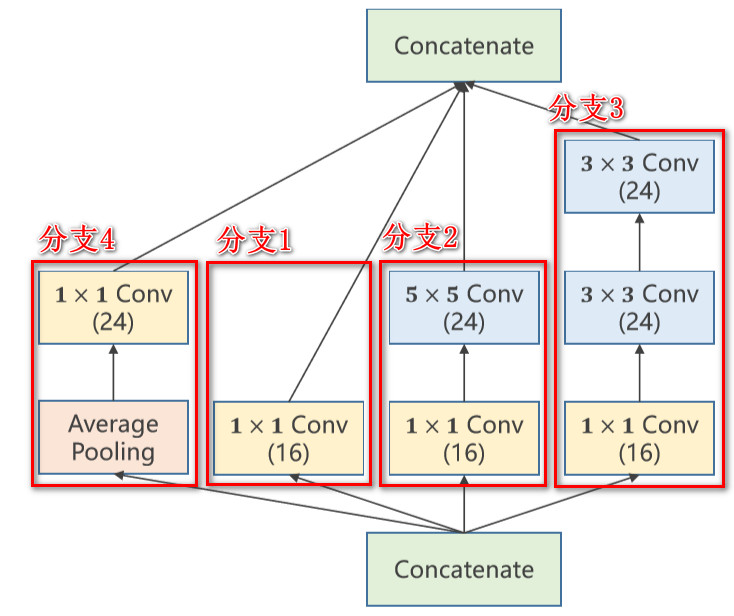
自學筆記 課程老師:劉二大人 河北工業大學教師 https://liuii.github.io 課程來源:https://www.bilibili.com/video/BV1Y7411d7Ys 十一、Implementation_of_Inception_Module 先看一下Inception_Module模塊的圖,課上老師按照下面的圖進行的類的構建,然后封裝,碼代碼時,是按照圖中標注的分支1&...


freemarker + ItextRender 根據模板生成PDF文件
1. 制作模板 2. 獲取模板,并將所獲取的數據加載生成html文件 2. 生成PDF文件 其中由兩個地方需要注意,都是關于獲取文件路徑的問題,由于項目部署的時候是打包成jar包形式,所以在開發過程中時直接安照傳統的獲取方法沒有一點文件,但是當打包后部署,總是出錯。于是參考網上文章,先將文件讀出來到項目的臨時目錄下,然后再按正常方式加載該臨時文件; 還有一個問題至今沒有解決,就是關于生成PDF文件...
電腦空間不夠了?教你一個小秒招快速清理 Docker 占用的磁盤空間!
Docker 很占用空間,每當我們運行容器、拉取鏡像、部署應用、構建自己的鏡像時,我們的磁盤空間會被大量占用。 如果你也被這個問題所困擾,咱們就一起看一下 Docker 是如何使用磁盤空間的,以及如何回收。 docker 占用的空間可以通過下面的命令查看: TYPE 列出了docker 使用磁盤的 4 種類型: Images:所有鏡像占用的空間,包括拉取下來的鏡像,和本地構建的。 Con...
猜你喜歡

requests實現全自動PPT模板
http://www.1ppt.com/moban/ 可以免費的下載PPT模板,當然如果要人工一個個下,還是挺麻煩的,我們可以利用requests輕松下載 訪問這個主頁,我們可以看到下面的樣式 點每一個PPT模板的圖片,我們可以進入到詳細的信息頁面,翻到下面,我們可以看到對應的下載地址 點擊這個下載的按鈕,我們便可以下載對應的PPT壓縮包 那我們就開始做吧 首先,查看網頁的源代碼,我們可以看到每一...
Linux C系統編程-線程互斥鎖(四)
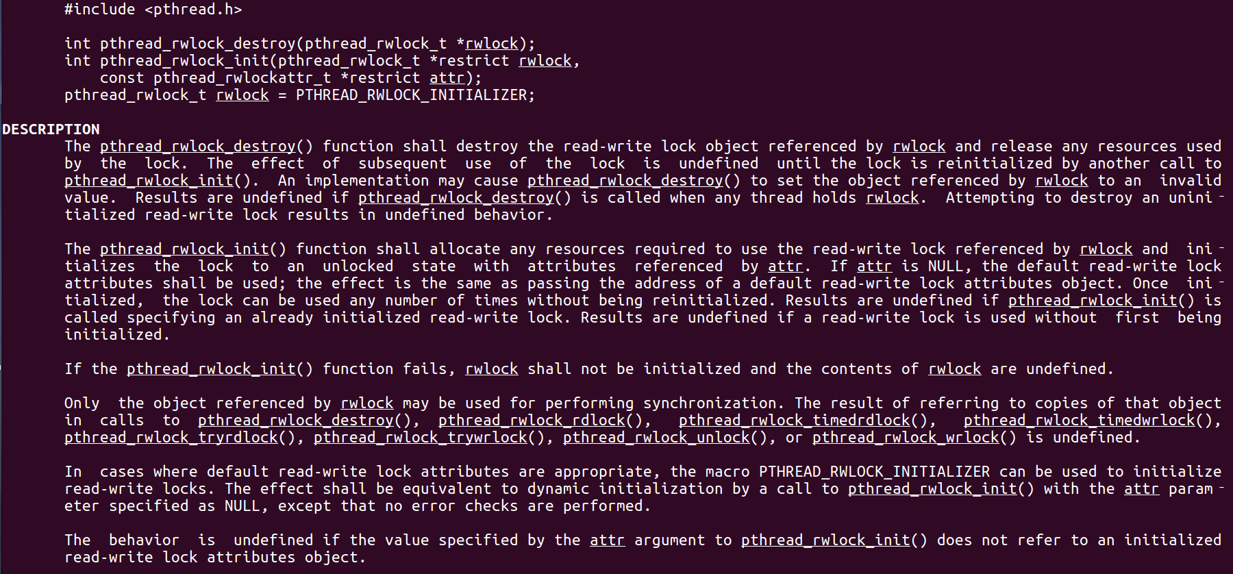
互斥鎖 互斥鎖也是屬于線程之間處理同步互斥方式,有上鎖/解鎖兩種狀態。 互斥鎖函數接口 1)初始化互斥鎖 pthread_mutex_init() man 3 pthread_mutex_init (找不到的情況下首先 sudo apt-get install glibc-doc sudo apt-get install manpages-posix-dev) 動態初始化 int pthread_...
統計學習方法 - 樸素貝葉斯
引入問題:一機器在良好狀態生產合格產品幾率是 90%,在故障狀態生產合格產品幾率是 30%,機器良好的概率是 75%。若一日第一件產品是合格品,那么此日機器良好的概率是多少。 貝葉斯模型 生成模型與判別模型 判別模型,即要判斷這個東西到底是哪一類,也就是要求y,那就用給定的x去預測。 生成模型,是要生成一個模型,那就是誰根據什么生成了模型,誰就是類別y,根據的內容就是x 以上述例子,判斷一個生產出...

styled-components —— React 中的 CSS 最佳實踐
https://zhuanlan.zhihu.com/p/29344146 Styled-components 是目前 React 樣式方案中最受關注的一種,它既具備了 css-in-js 的模塊化與參數化優點,又完全使用CSS的書寫習慣,不會引起額外的學習成本。本文是 styled-components 作者之一 Max Stoiber 所寫,首先總結了前端組件化樣式中的最佳實踐原則,然后在此基...