Python極簡入門(三)
廣播Broadcasting
廣播可以讓Numpy不同大小的矩陣進行數學計算,e.g.把一個向量加到矩陣每一行
import numpy as np

# We will add the vector v to each row of the matrix x,
# storing the result in the matrix y
x = np.array([[1,2,3], [4,5,6], [7,8,9], [10, 11, 12]])
v = np.array([1, 0, 1])
y = np.empty_like(x)   # Create an empty matrix with the same shape as x

# Add the vector v to each row of the matrix x with an explicit loop
for i in range(4):
    y[i, :] = x[i, :] + v

# Now y is the following
# [[ 2  2  4]
#  [ 5  5  7]
#  [ 8  8 10]
#  [11 11 13]]
print y
但是當x非常大,上述運算就會很慢,另一種思路:
import numpy as np

# We will add the vector v to each row of the matrix x,
# storing the result in the matrix y
x = np.array([[1,2,3], [4,5,6], [7,8,9], [10, 11, 12]])
v = np.array([1, 0, 1])
vv = np.tile(v, (4, 1))  # Stack 4 copies of v on top of each other
print vv                 # Prints "[[1 0 1]
                         #          [1 0 1]
                         #          [1 0 1]
                         #          [1 0 1]]"
y = x + vv  # Add x and vv elementwise
print y  # Prints "[[ 2  2  4
         #          [ 5  5  7]
         #          [ 8  8 10]
         #          [11 11 13]]"
使用numpy的廣播機制就很直接了:
import numpy as np

# We will add the vector v to each row of the matrix x,
# storing the result in the matrix y
x = np.array([[1,2,3], [4,5,6], [7,8,9], [10, 11, 12]])
v = np.array([1, 0, 1])
y = x + v  # Add v to each row of x using broadcasting
print y  # Prints "[[ 2  2  4]
         #          [ 5  5  7]
         #          [ 8  8 10]
         #          [11 11 13]]"
對兩個數組使用廣播也要遵守一定的規則:
1)如果數組的秩不同,使用1將秩較小的數組進行擴展,知道兩個數組的尺寸一樣。
2)如果兩個數組某個維度的長度一樣或者其中一個數組在某維度上長度為1,那么我們說兩個數組在該維度上是相容的。
3)如果兩個數組在所有維度上都是相容的,他們就能使用廣播。
4)如果兩個數組尺寸不同,廣播之后,兩個數組的尺寸將和較大的尺寸一樣。
5)在任何一個維度是哪個,如果一個數組長度為1,另一個大于1,那么在該維度上就好像對第一個數組進行復制。
以下是一些廣播的使用:
import numpy as np

# Compute outer product of vectors
v = np.array([1,2,3])  # v has shape (3,)
w = np.array([4,5])    # w has shape (2,)
# To compute an outer product, we first reshape v to be a column
# vector of shape (3, 1); we can then broadcast it against w to yield
# an output of shape (3, 2), which is the outer product of v and w:
# [[ 4  5]
#  [ 8 10]
#  [12 15]]
print np.reshape(v, (3, 1)) * w

# Add a vector to each row of a matrix
x = np.array([[1,2,3], [4,5,6]])
# x has shape (2, 3) and v has shape (3,) so they broadcast to (2, 3),
# giving the following matrix:
# [[2 4 6]
#  [5 7 9]]
print x + v

# Add a vector to each column of a matrix
# x has shape (2, 3) and w has shape (2,).
# If we transpose x then it has shape (3, 2) and can be broadcast
# against w to yield a result of shape (3, 2); transposing this result
# yields the final result of shape (2, 3) which is the matrix x with
# the vector w added to each column. Gives the following matrix:
# [[ 5  6  7]
#  [ 9 10 11]]
print (x.T + w).T

# Another solution is to reshape w to be a row vector of shape (2, 1);
# we can then broadcast it directly against x to produce the same
# output.
print x + np.reshape(w, (2, 1))

# Multiply a matrix by a constant:
# x has shape (2, 3). Numpy treats scalars as arrays of shape ();
# these can be broadcast together to shape (2, 3), producing the
# following array:
# [[ 2  4  6]
#  [ 8 10 12]]
print x * 2
SciPy
SciPy基于Numpy,提供大量計算和操作數組的函數,對于不同類型的科學和工程計算很有用。
圖像操作:
提供一些操作圖像的基本函數,例:將圖像從硬盤讀入數組;數組數據寫入硬盤成為圖像。
from scipy.misc import imread, imsave, imresize

# Read an JPEG image into a numpy array
img = imread('assets/cat.jpg')
print img.dtype, img.shape  # Prints "uint8 (400, 248, 3)"

# We can tint the image by scaling each of the color channels
# by a different scalar constant. The image has shape (400, 248, 3);
# we multiply it by the array [1, 0.95, 0.9] of shape (3,);
# numpy broadcasting means that this leaves the red channel unchanged,
# and multiplies the green and blue channels by 0.95 and 0.9
# respectively.
img_tinted = img * [1, 0.95, 0.9]

# Resize the tinted image to be 300 by 300 pixels.
img_tinted = imresize(img_tinted, (300, 300))

# Write the tinted image back to disk
imsave('assets/cat_tinted.jpg', img_tinted)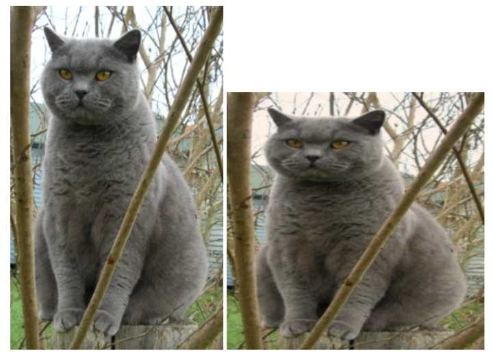
MATLAB文件
scipy.io,loadmat和scipy.io.savemat可以讀寫MATLAB文件。
點之間的距離
scipy的函數scipy.spatial.distance.pdist能夠計算集合中所有兩點之間的距離:
import numpy as np
from scipy.spatial.distance import pdist, squareform

# Create the following array where each row is a point in 2D space:
# [[0 1]
#  [1 0]
#  [2 0]]
x = np.array([[0, 1], [1, 0], [2, 0]])
print x

# Compute the Euclidean distance between all rows of x.
# d[i, j] is the Euclidean distance between x[i, :] and x[j, :],
# and d is the following array:
# [[ 0.          1.41421356  2.23606798]
#  [ 1.41421356  0.          1.        ]
#  [ 2.23606798  1.          0.        ]]
d = squareform(pdist(x, 'euclidean'))
print dMatplotlib
Matplotlib是一個做圖庫,這里只介紹matplotlib.pyplot模塊,功能和MATLAB作圖功能類似。
繪圖
matplotlib庫中最重要的函數是Plot,該函數允許你做出2D圖形:
import numpy as np
import matplotlib.pyplot as plt

# Compute the x and y coordinates for points on a sine curve
x = np.arange(0, 3 * np.pi, 0.1)
y = np.sin(x)

# Plot the points using matplotlib
plt.plot(x, y)
plt.show()  # You must call plt.show() to make graphics appear.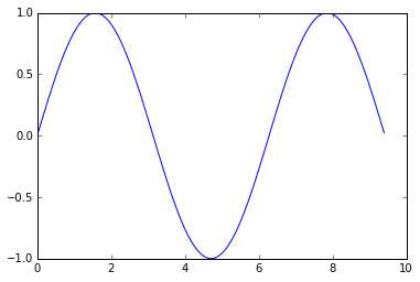
還可以加標簽,坐標軸標志等:
import numpy as np
import matplotlib.pyplot as plt

# Compute the x and y coordinates for points on sine and cosine curves
x = np.arange(0, 3 * np.pi, 0.1)
y_sin = np.sin(x)
y_cos = np.cos(x)

# Plot the points using matplotlib
plt.plot(x, y_sin)
plt.plot(x, y_cos)
plt.xlabel('x axis label')
plt.ylabel('y axis label')
plt.title('Sine and Cosine')
plt.legend(['Sine', 'Cosine'])
plt.show()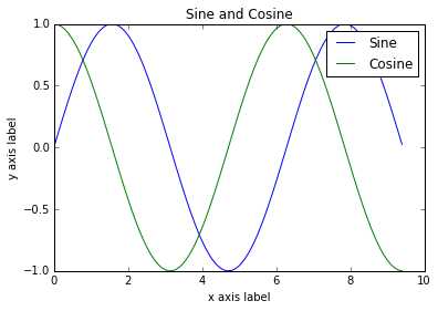
繪制多個圖像
使用subplot函數在一幅圖中畫不同的東西:
import numpy as np
import matplotlib.pyplot as plt

# Compute the x and y coordinates for points on sine and cosine curves
x = np.arange(0, 3 * np.pi, 0.1)
y_sin = np.sin(x)
y_cos = np.cos(x)

# Set up a subplot grid that has height 2 and width 1,
# and set the first such subplot as active.
plt.subplot(2, 1, 1)

# Make the first plot
plt.plot(x, y_sin)
plt.title('Sine')

# Set the second subplot as active, and make the second plot.
plt.subplot(2, 1, 2)
plt.plot(x, y_cos)
plt.title('Cosine')

# Show the figure.
plt.show()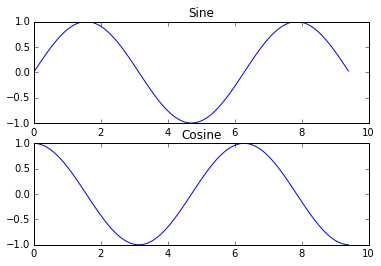
圖像
使用imshow函數顯示圖像:
import numpy as np
from scipy.misc import imread, imresize
import matplotlib.pyplot as plt

img = imread('assets/cat.jpg')
img_tinted = img * [1, 0.95, 0.9]

# Show the original image
plt.subplot(1, 2, 1)
plt.imshow(img)

# Show the tinted image
plt.subplot(1, 2, 2)

# A slight gotcha with imshow is that it might give strange results
# if presented with data that is not uint8. To work around this, we
# explicitly cast the image to uint8 before displaying it.
plt.imshow(np.uint8(img_tinted))
plt.show()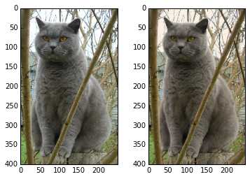
參考https://zhuanlan.zhihu.com/p/20878530?refer=intelligentunit
智能推薦
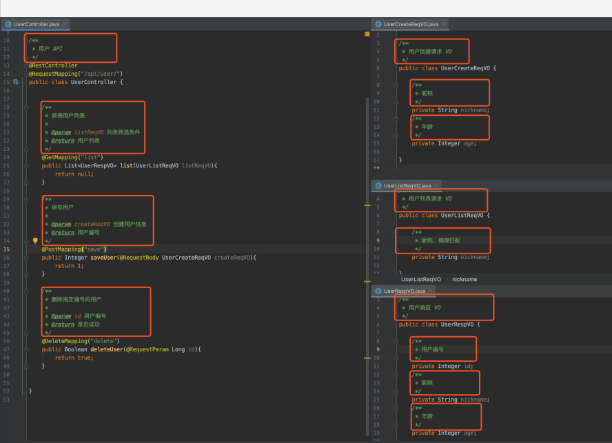
JApiDocs 極簡入門
JApiDocs java api接口文檔 源碼地址: https://github.com/YeDaxia/JApiDocs 1 、引入依賴 2 、創建 JApiDocs 配置 創建 TestJApiDocs 類,作為 JApiDocs 的配置,生成接口文檔 : 2 、代碼注釋 JApiDocs 是通過解析 Controller 源碼上的 Java 注釋,所以我們需要在相關的類、方法、屬性上,進...

Dockerfile極簡入門
Docker會依據Dockerfile內部的指令來在基礎鏡像上構建新的內容。 1. FROM 指明構建的新鏡像是來自于哪個基礎鏡像,例如: 2. MAINTAINER 指明鏡像維護著及其聯系方式(一般是郵箱地址),例如: 不過,MAINTAINER并不推薦使用,更推薦使用LABEL來指定鏡像作者,例如:LABEL maintainer="edisonzhou.cn" 3. RU...


freemarker + ItextRender 根據模板生成PDF文件
1. 制作模板 2. 獲取模板,并將所獲取的數據加載生成html文件 2. 生成PDF文件 其中由兩個地方需要注意,都是關于獲取文件路徑的問題,由于項目部署的時候是打包成jar包形式,所以在開發過程中時直接安照傳統的獲取方法沒有一點文件,但是當打包后部署,總是出錯。于是參考網上文章,先將文件讀出來到項目的臨時目錄下,然后再按正常方式加載該臨時文件; 還有一個問題至今沒有解決,就是關于生成PDF文件...
電腦空間不夠了?教你一個小秒招快速清理 Docker 占用的磁盤空間!
Docker 很占用空間,每當我們運行容器、拉取鏡像、部署應用、構建自己的鏡像時,我們的磁盤空間會被大量占用。 如果你也被這個問題所困擾,咱們就一起看一下 Docker 是如何使用磁盤空間的,以及如何回收。 docker 占用的空間可以通過下面的命令查看: TYPE 列出了docker 使用磁盤的 4 種類型: Images:所有鏡像占用的空間,包括拉取下來的鏡像,和本地構建的。 Con...
猜你喜歡

requests實現全自動PPT模板
http://www.1ppt.com/moban/ 可以免費的下載PPT模板,當然如果要人工一個個下,還是挺麻煩的,我們可以利用requests輕松下載 訪問這個主頁,我們可以看到下面的樣式 點每一個PPT模板的圖片,我們可以進入到詳細的信息頁面,翻到下面,我們可以看到對應的下載地址 點擊這個下載的按鈕,我們便可以下載對應的PPT壓縮包 那我們就開始做吧 首先,查看網頁的源代碼,我們可以看到每一...
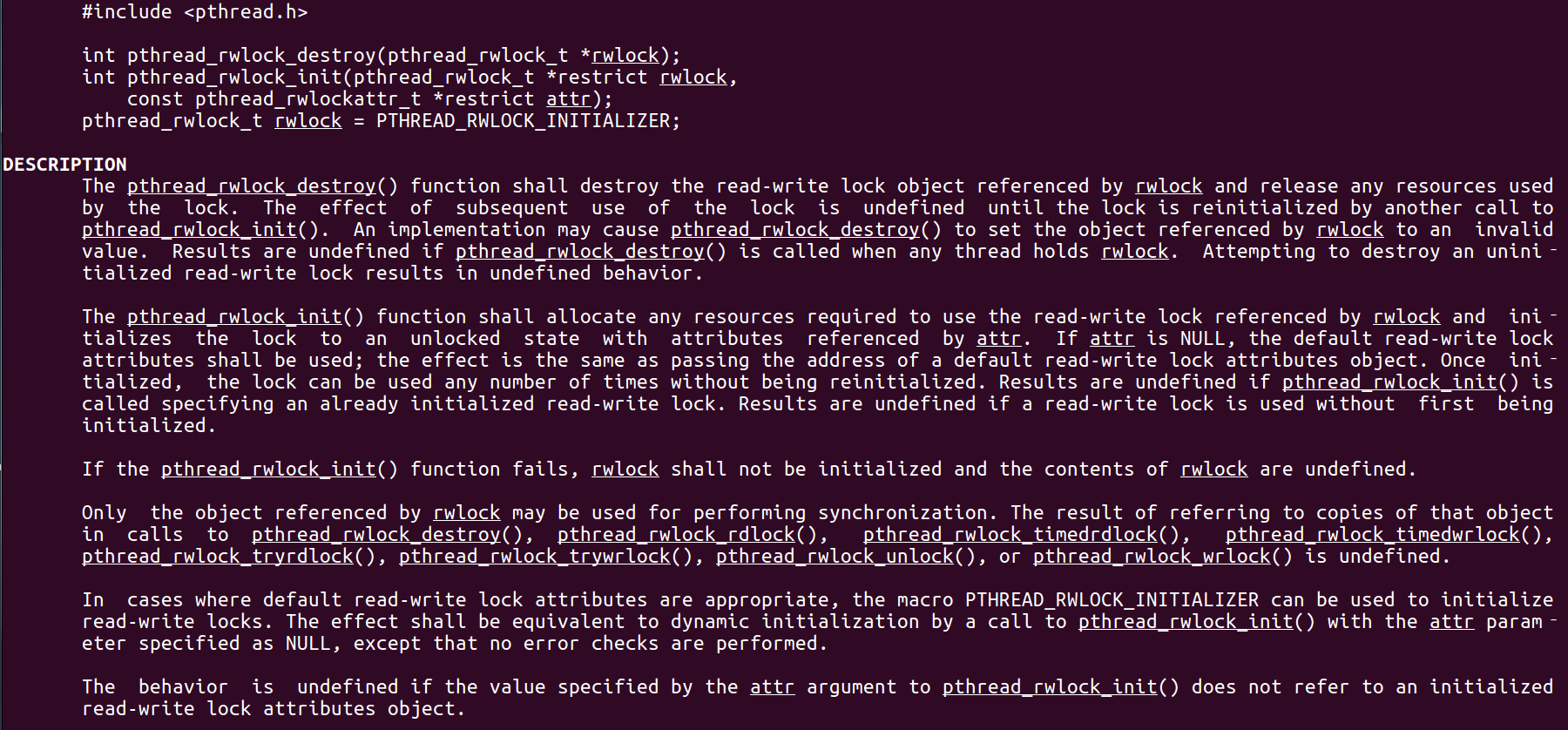
Linux C系統編程-線程互斥鎖(四)
互斥鎖 互斥鎖也是屬于線程之間處理同步互斥方式,有上鎖/解鎖兩種狀態。 互斥鎖函數接口 1)初始化互斥鎖 pthread_mutex_init() man 3 pthread_mutex_init (找不到的情況下首先 sudo apt-get install glibc-doc sudo apt-get install manpages-posix-dev) 動態初始化 int pthread_...
統計學習方法 - 樸素貝葉斯
引入問題:一機器在良好狀態生產合格產品幾率是 90%,在故障狀態生產合格產品幾率是 30%,機器良好的概率是 75%。若一日第一件產品是合格品,那么此日機器良好的概率是多少。 貝葉斯模型 生成模型與判別模型 判別模型,即要判斷這個東西到底是哪一類,也就是要求y,那就用給定的x去預測。 生成模型,是要生成一個模型,那就是誰根據什么生成了模型,誰就是類別y,根據的內容就是x 以上述例子,判斷一個生產出...

styled-components —— React 中的 CSS 最佳實踐
https://zhuanlan.zhihu.com/p/29344146 Styled-components 是目前 React 樣式方案中最受關注的一種,它既具備了 css-in-js 的模塊化與參數化優點,又完全使用CSS的書寫習慣,不會引起額外的學習成本。本文是 styled-components 作者之一 Max Stoiber 所寫,首先總結了前端組件化樣式中的最佳實踐原則,然后在此基...