Andrew Ng Deep Learning 第四課 第一周
Andrew Ng Deep Learning 第四課 第一周
前言
網易云課堂(雙語字幕,不卡):https://mooc.study.163.com/smartSpec/detail/1001319001.htmcourseId=1004570029、
Coursera(貴):https://www.coursera.org/specializations/deep-learning
本人初學者,先在網易云課堂上看網課,再去Coursera上做作業,開博客以記錄,文章中引用圖片皆為課程中所截。
題目轉載至:http://www.cnblogs.com/hezhiyao/p/7810725.html
編程作業所需庫:鏈接:https://pan.baidu.com/s/1aS1Oia2fskemBHHEMnSepw 密碼:66gd
卷積神經網絡CNN
邊緣檢測
卷積算法
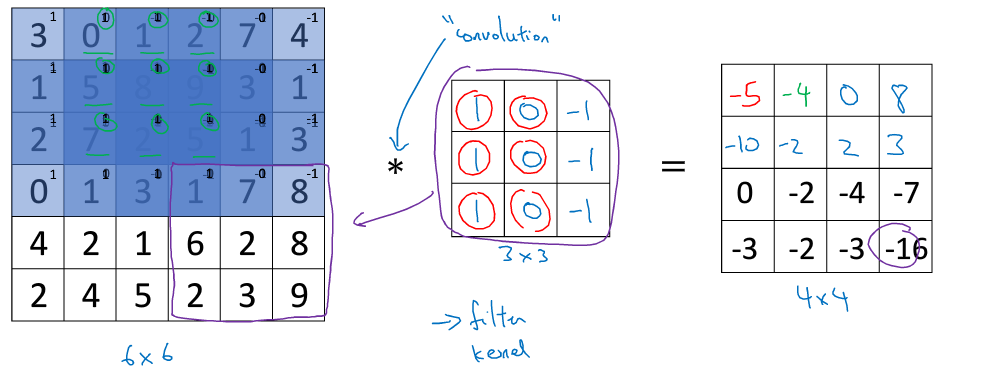
Tips:一個n×n的矩陣,卷積一個f×f的矩陣(稱為過濾器),得到一個(n-f+1)×(n-f+1)矩陣,算法:將過濾器覆蓋上初始矩陣,相應位置相應乘積后累加,得到該位置的數后向右移動,移動到盡頭后移動至下一行開頭,第一個格子為31+11+21+00+50+70+1*-1+8*-1+2*-1=-5,第二個格子即將3×3過濾器右移一格
Padding
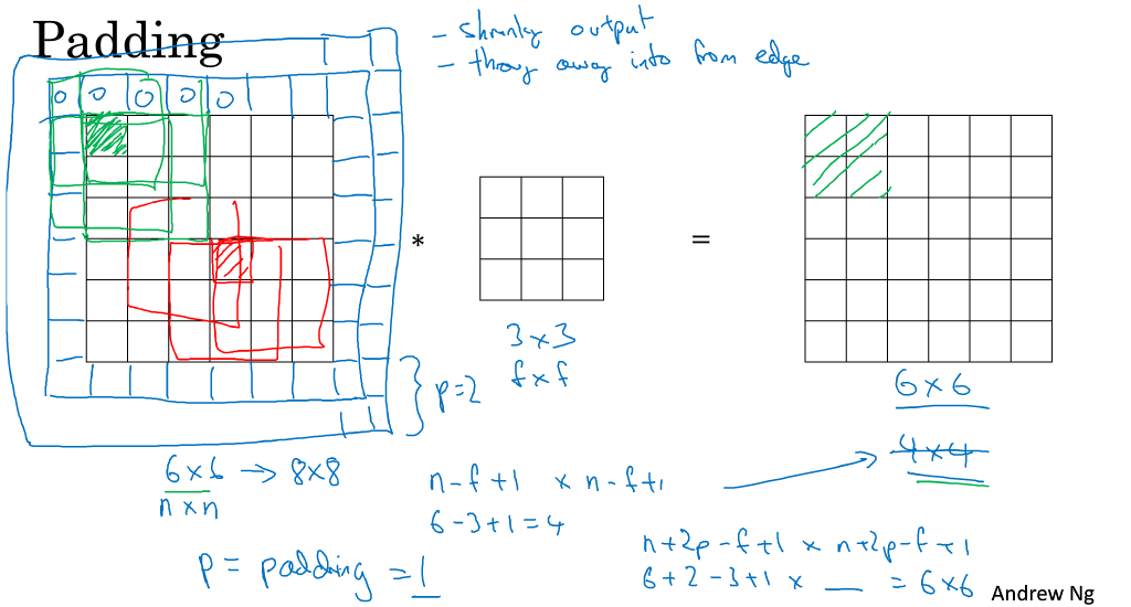
Tips:簡單來說就是多出去p行,多出去的部分均為0,這樣能使每個格子被應用到的次數更為平均,這樣得到的矩陣結果維度為(n+2p-f+1)×(n+2p-f+1)
卷積步長
Tips:步長s為2的情況,得到矩陣為((n+2p-f)/s+1)×((n+2p-f)/2+1)
簡單卷積網絡總結示例
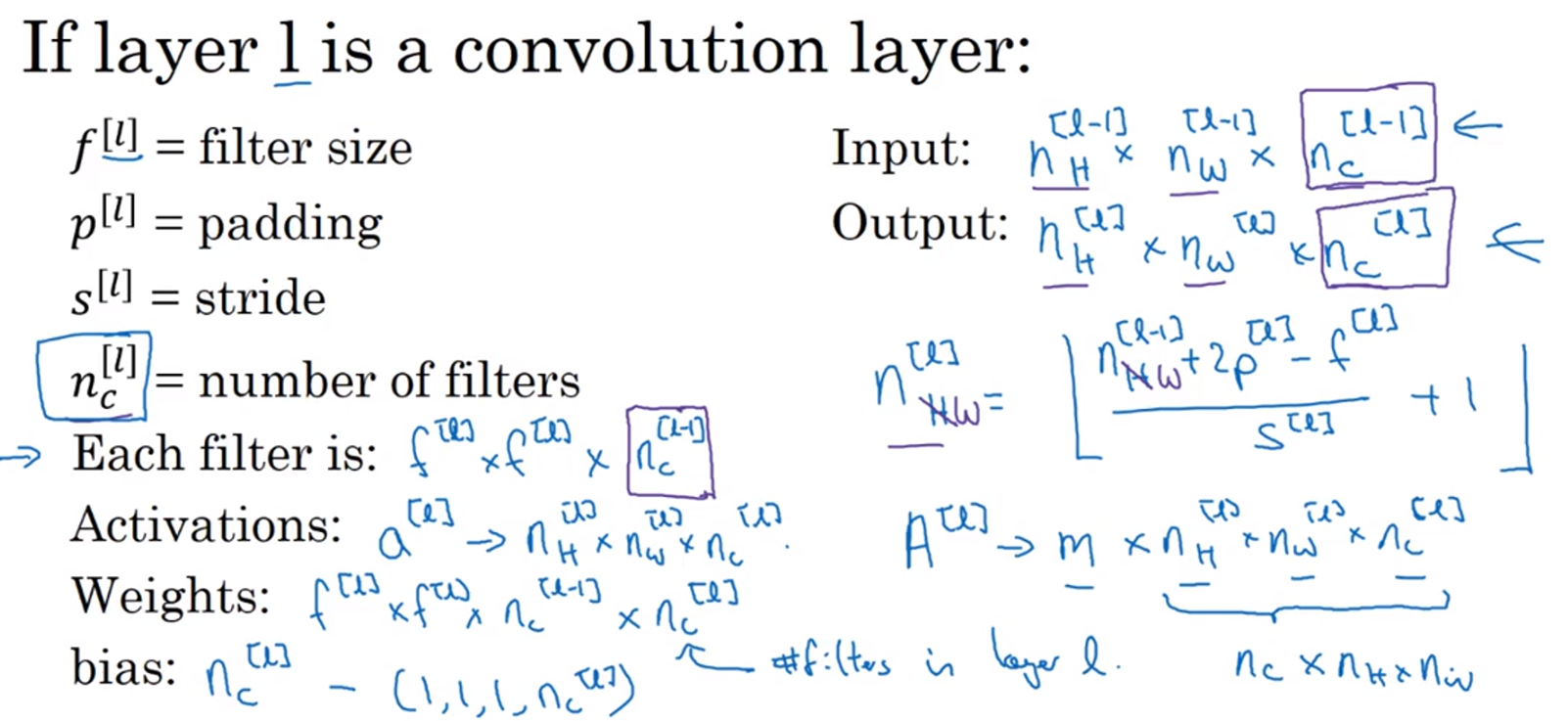
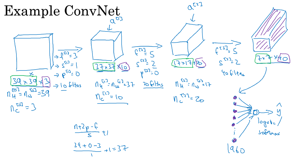
Tips:第一個卷積層有10個過濾器,得到10個通道堆疊,這就是37×37×10中10的由來
池化層
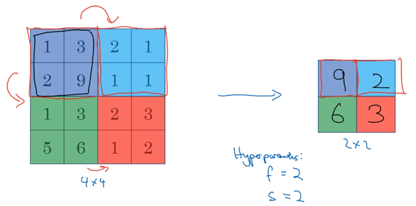
Tips:最大池化層,例如從2×2中取出最大值,然后根據步幅s移動,(n-s)/2+1
卷積神經網絡示例
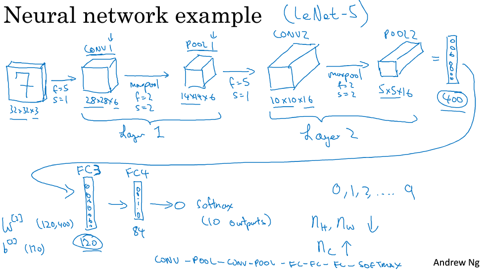 Tips:最后layer2卷積層和池化層后得到5×5×16,將其舒展程400*1向量,最后再經過FC3與FC4(稱為全連接層,即每個結點都與上一層的每一個結點相連)后運用softmax進行預測
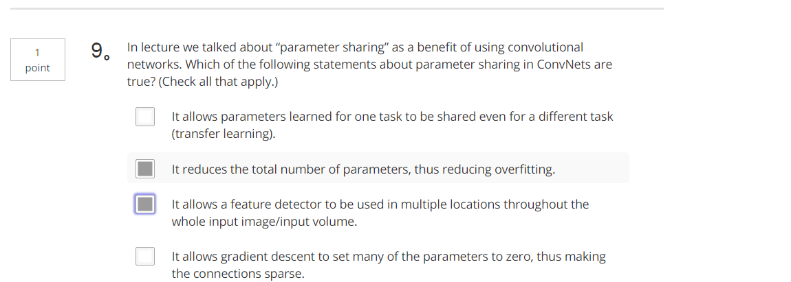
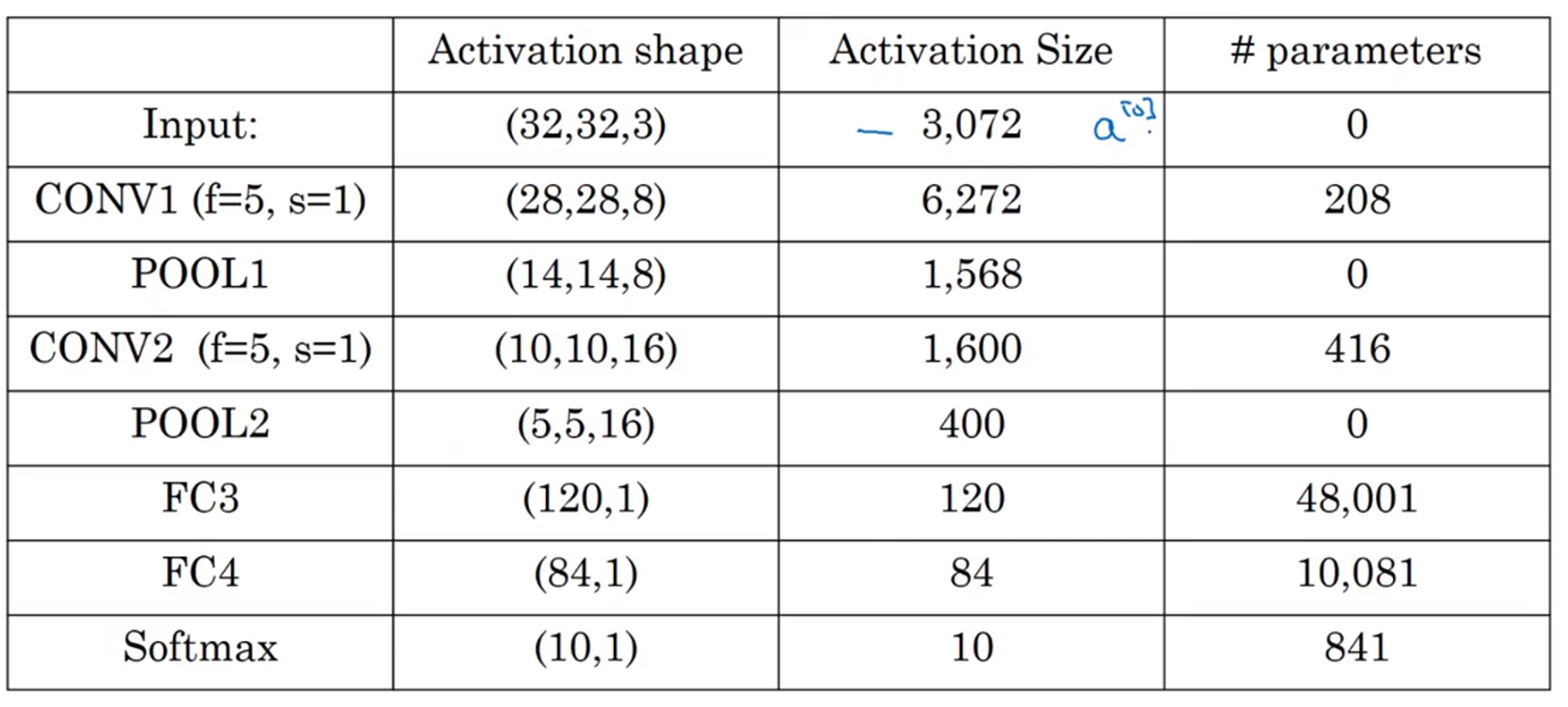 Tips:顯而易見的是卷積網絡使我們需要的參數變少了,池化層是不需要參數只需要f、s和p超參數,卷積層需要參數即為過濾器的參數,例如卷積層1參數為(5×5×8)+8(此處8為偏置bias),例如全連接層三參數為(120,400)+1
編程作業
底層搭建
import numpy as np
import h5py
import matplotlib.pyplot as plt

%matplotlib inline
plt.rcParams['figure.figsize'] = (5.0, 4.0) # set default size of plots
plt.rcParams['image.interpolation'] = 'nearest'
plt.rcParams['image.cmap'] = 'gray'

%load_ext autoreload
%autoreload 2

np.random.seed(1)
def zero_pad(X, pad):
    """
    把數據集X的圖像邊界全部使用0來擴充pad個寬度和高度。

    參數:
        X - 圖像數據集,維度為(樣本數,圖像高度,圖像寬度,圖像通道數)
        pad - 整數,每個圖像在垂直和水平維度上的填充量
    返回:
        X_paded - 擴充后的圖像數據集,維度為(樣本數,圖像高度 + 2*pad,圖像寬度 + 2*pad,圖像通道數)

    """

    ### START CODE HERE ### (≈ 1 line)
    X_pad = np.pad(X,((0,0),(pad,pad),(pad,pad),(0,0)),'constant', constant_values=(0,0) )
    ### END CODE HERE ###

    return X_pad
def conv_single_step(a_slice_prev,W,b):
    """
    在前一層的**輸出的一個片段上應用一個由參數W定義的過濾器。
    這里切片大小和過濾器大小相同

    參數:
        a_slice_prev - 輸入數據的一個片段,維度為(過濾器大小,過濾器大小,上一通道數)
        W - 權重參數,包含在了一個矩陣中,維度為(過濾器大小,過濾器大小,上一通道數)
        b - 偏置參數,包含在了一個矩陣中,維度為(1,1,1)

    返回:
        Z - 在輸入數據的片X上卷積滑動窗口(w,b)的結果。
    """
    ### START CODE HERE ### (≈ 2 lines of code)
    # Element-wise product between a_slice and W. Do not add the bias yet.
    Z=np.multiply(W,a_slice_prev)
    #Add bias b to Z. Cast b to a float() so that Z results in a scalar value.
    Z=Z+float(b)
    # Sum over all entries of the volume s.
    Z=np.sum(Z)
    ### END CODE HERE ###

    return Z

def conv_forward(A_prev, W, b, hparameters):
    """
    實現卷積函數的前向傳播

    參數:
        A_prev - 上一層的**輸出矩陣,維度為(m, n_H_prev, n_W_prev, n_C_prev),(樣本數量,上一層圖像的高度,上一層圖像的寬度,上一層過濾器數量)
        W - 權重矩陣,維度為(f, f, n_C_prev, n_C),(過濾器大小,過濾器大小,上一層的過濾器數量,這一層的過濾器數量)
        b - 偏置矩陣,維度為(1, 1, 1, n_C),(1,1,1,這一層的過濾器數量)
        hparameters - 包含了"stride"與 "pad"的超參數字典。

    返回:
        Z - 卷積輸出,維度為(m, n_H, n_W, n_C),(樣本數,圖像的高度,圖像的寬度,過濾器數量)
        cache - 緩存了一些反向傳播函數conv_backward()需要的一些數據
    """
    ### START CODE HERE ###
    # Retrieve dimensions from A_prev's shape (≈1 line)  從 A_prev 的形狀中檢索維度
    (m, n_H_prev, n_W_prev, n_C_prev)=A_prev.shape

    # Retrieve dimensions from W's shape (≈1 line)
    (f, f, n_C_prev, n_C)=W.shape

    # Retrieve information from "hparameters" (≈2 lines)
    stride=hparameters['stride']
    pad=hparameters['pad']

    # Compute the dimensions of the CONV output volume using the formula given above. Hint: use int() to floor. (≈2 lines)
    n_H=int((n_H_prev+2*pad-f)/stride+1)
    n_W=int((n_W_prev+2*pad-f)/stride+1)

    # Initialize the output volume Z with zeros. (≈1 line)
    Z=np.zeros((m,n_H,n_W,n_C))

    # Create A_prev_pad by padding A_prev
    A_prev_pad=zero_pad(A_prev, pad)

    for i in range(m):                               # loop over the batch of training examples
        a_prev_pad = A_prev_pad[i]                   # Select ith training example's padded activation
        for h in range(n_H):                           # loop over vertical axis of the output volume
            for w in range(n_W):                       # loop over horizontal axis of the output volume
                for c in range(n_C):                   # loop over channels (= #filters) of the output volume

                    # Find the corners of the current "slice" (≈4 lines)
                    vert_start=h*stride
                    vert_end=vert_start+f
                    horiz_start=w*stride
                    horiz_end=horiz_start+f

                    # Use the corners to define the (3D) slice of a_prev_pad (See Hint above the cell). (≈1 line)
                    a_pad=a_prev_pad[vert_start:vert_end,horiz_start:horiz_end,:]

                    # Convolve the (3D) slice with the correct filter W and bias b, to get back one output neuron. (≈1 line)
                    Z[i][h][w][c]=conv_single_step(a_pad,W[:,:,:,c],b[0,0,0,c])

    ### END CODE HERE ###

    # Making sure your output shape is correct
    assert(Z.shape == (m, n_H, n_W, n_C))

    # Save information in "cache" for the backprop
    cache = (A_prev, W, b, hparameters)

    return Z, cache
def pool_forward(A_prev,hparameters,mode="max"):
    """
    實現池化層的前向傳播

    參數:
        A_prev - 輸入數據,維度為(m, n_H_prev, n_W_prev, n_C_prev)
        hparameters - 包含了 "f" 和 "stride"的超參數字典
        mode - 模式選擇【"max" | "average"】

    返回:
        A - 池化層的輸出,維度為 (m, n_H, n_W, n_C)
        cache - 存儲了一些反向傳播需要用到的值,包含了輸入和超參數的字典。
    """
    # Retrieve dimensions from the input shape
    (m, n_H_prev, n_W_prev, n_C_prev) = A_prev.shape

    # Retrieve hyperparameters from "hparameters"
    f = hparameters["f"]
    stride = hparameters["stride"]

    # Define the dimensions of the output
    n_H = int(1 + (n_H_prev - f) / stride)
    n_W = int(1 + (n_W_prev - f) / stride)
    n_C = n_C_prev

    # Initialize output matrix A
    A = np.zeros((m, n_H, n_W, n_C))

    ### START CODE HERE ###
    for i in range(m):                         # loop over the training examples
        for h in range(n_H):                     # loop on the vertical axis of the output volume
            for w in range(n_W):                 # loop on the horizontal axis of the output volume
                for c in range (n_C):            # loop over the channels of the output volume

                    # Find the corners of the current "slice" (≈4 lines)
                    vert_start=h*stride
                    vert_end=vert_start+f
                    horiz_start=w*stride
                    horiz_end=horiz_start+f

                    # Use the corners to define the current slice on the ith training example of A_prev, channel c. (≈1 line)
                    a_prev=A_prev[i,vert_start:vert_end,horiz_start:horiz_end,c]
                    # Compute the pooling operation on the slice. Use an if statment to differentiate the modes. Use np.max/np.mean.
                    if (mode=='max'):
                        A[i,h,w,c]=np.max(a_prev)
                    else:
                        A[i,h,w,c]=np.mean(a_prev)
    ### END CODE HERE ###

    # Store the input and hparameters in "cache" for pool_backward()
    cache = (A_prev, hparameters)

    # Making sure your output shape is correct
    assert(A.shape == (m, n_H, n_W, n_C))

    return A, cache
TensorFlow版本
import math
import numpy as np
import h5py
import matplotlib.pyplot as plt
import matplotlib.image as mpimg
import tensorflow as tf
import tf_utils
from tensorflow.python.framework import ops
import cnn_utils
%matplotlib inline
np.random.seed(1)
def create_placeholders(n_H0, n_W0, n_C0, n_y):
"""
為session創建占位符
參數:
n_H0 - 實數,輸入圖像的高度
n_W0 - 實數,輸入圖像的寬度
n_C0 - 實數,輸入的通道數
n_y - 實數,分類數
輸出:
X - 輸入數據的占位符,維度為[None, n_H0, n_W0, n_C0],類型為"float"
Y - 輸入數據的標簽的占位符,維度為[None, n_y],維度為"float"
"""
X = tf.placeholder(tf.float32,[None, n_H0, n_W0, n_C0])
Y = tf.placeholder(tf.float32,[None, n_y])
return X,Y
def initialize_parameters():
"""
初始化權值矩陣,這里我們把權值矩陣硬編碼:
W1 : [4, 4, 3, 8]
W2 : [2, 2, 8, 16]
返回:
包含了tensor類型的W1、W2的字典
"""
tf.set_random_seed(1)
W1 = tf.get_variable("W1",[4,4,3,8],initializer=tf.contrib.layers.xavier_initializer(seed=0))
W2 = tf.get_variable("W2",[2,2,8,16],initializer=tf.contrib.layers.xavier_initializer(seed=0))
parameters = {"W1": W1,
"W2": W2}
return parameters
def forward_propagation(X,parameters):
"""
實現前向傳播
CONV2D -> RELU -> MAXPOOL -> CONV2D -> RELU -> MAXPOOL -> FLATTEN -> FULLYCONNECTED
參數:
X - 輸入數據的placeholder,維度為(輸入節點數量,樣本數量)
parameters - 包含了“W1”和“W2”的python字典。
返回:
Z3 - 最后一個LINEAR節點的輸出
"""
# Retrieve the parameters from the dictionary "parameters"
W1 = parameters['W1']* np.sqrt(2)
W2 = parameters['W2']* np.sqrt(2 / 192)
### START CODE HERE ###
# CONV2D: stride of 1, padding 'SAME'
Z1=tf.nn.conv2d(X,W1,strides=[1,1,1,1],padding='SAME')
# RELU
A1 = tf.nn.relu(Z1)
# MAXPOOL: window 8x8, sride 8, padding 'SAME'
P1 = tf.nn.max_pool(A1,ksize=[1,8,8,1],strides=[1,8,8,1],padding="SAME")
# CONV2D: filters W2, stride 1, padding 'SAME'
Z2 = tf.nn.conv2d(P1,W2,strides=[1,1,1,1],padding="SAME")
# RELU
A2 = tf.nn.relu(Z2)
# MAXPOOL: window 4x4, stride 4, padding 'SAME'
P2 = tf.nn.max_pool(A2,ksize=[1,4,4,1],strides=[1,4,4,1],padding="SAME")
# FLATTEN
P = tf.contrib.layers.flatten(P2)
# FULLY-CONNECTED without non-linear activation function (not not call softmax).
# 6 neurons in output layer. Hint: one of the arguments should be "activation_fn=None"
Z3 = tf.contrib.layers.fully_connected(P,6,activation_fn=None)
### END CODE HERE ###
return Z3
def compute_cost(Z3,Y):
"""
計算成本
參數:
Z3 - 正向傳播最后一個LINEAR節點的輸出,維度為(6,樣本數)。
Y - 標簽向量的placeholder,和Z3的維度相同
返回:
cost - 計算后的成本
"""
cost = tf.reduce_mean(tf.nn.softmax_cross_entropy_with_logits(logits=Z3,labels=Y))
return cost
def model(X_train, Y_train, X_test, Y_test, learning_rate=0.005,
num_epochs=1500,minibatch_size=64,print_cost=True,isPlot=True):
"""
使用TensorFlow實現三層的卷積神經網絡
CONV2D -> RELU -> MAXPOOL -> CONV2D -> RELU -> MAXPOOL -> FLATTEN -> FULLYCONNECTED
參數:
X_train - 訓練數據,維度為(None, 64, 64, 3)
Y_train - 訓練數據對應的標簽,維度為(None, n_y = 6)
X_test - 測試數據,維度為(None, 64, 64, 3)
Y_test - 訓練數據對應的標簽,維度為(None, n_y = 6)
learning_rate - 學習率
num_epochs - 遍歷整個數據集的次數
minibatch_size - 每個小批量數據塊的大小
print_cost - 是否打印成本值,每遍歷100次整個數據集打印一次
isPlot - 是否繪制圖譜
返回:
train_accuracy - 實數,訓練集的準確度
test_accuracy - 實數,測試集的準確度
parameters - 學習后的參數
"""
ops.reset_default_graph() # to be able to rerun the model without overwriting tf variables(能夠在不覆蓋 tf 變量的情況下重新運行模型)
tf.set_random_seed(1) # to keep results consistent (tensorflow seed)
seed = 3 # to keep results consistent (numpy seed)
(m, n_H0, n_W0, n_C0) = X_train.shape
n_y = Y_train.shape[1]
costs = [] # To keep track of the cost
# Create Placeholders of the correct shape
### START CODE HERE ### (1 line)
X , Y = create_placeholders(n_H0, n_W0, n_C0, n_y)
### END CODE HERE ###
# Initialize parameters
### START CODE HERE ### (1 line)
parameters=initialize_parameters()
### END CODE HERE ###
# Forward propagation: Build the forward propagation in the tensorflow graph
### START CODE HERE ### (1 line)
Z3=forward_propagation(X,parameters)
### END CODE HERE ###
# Cost function: Add cost function to tensorflow graph
### START CODE HERE ### (1 line)
cost = compute_cost(Z3,Y)
### END CODE HERE ###
# Backpropagation: Define the tensorflow optimizer. Use an AdamOptimizer that minimizes the cost.
### START CODE HERE ### (1 line)
optimizer = tf.train.AdamOptimizer(learning_rate=learning_rate).minimize(cost)
### END CODE HERE ###
# Initialize all the variables globally
init = tf.global_variables_initializer()
# Start the session to compute the tensorflow graph
with tf.Session() as sess:
# Run the initialization
sess.run(init)
# Do the training loop
for epoch in range(num_epochs):
minibatch_cost = 0
num_minibatches = int(m / minibatch_size) #獲取數據塊的數量
seed = seed + 1
minibatches = cnn_utils.random_mini_batches(X_train,Y_train,minibatch_size,seed)
for minibatch in minibatches:
# Select a minibatch
(minibatch_X, minibatch_Y) = minibatch
# IMPORTANT: The line that runs the graph on a minibatch. (在 minibatch 上運行圖的行。)
# Run the session to execute the optimizer and the cost, the feedict should contain a minibatch for (X,Y).
### START CODE HERE ### (1 line)
_ , temp_cost = sess.run([optimizer,cost],feed_dict={X:minibatch_X, Y:minibatch_Y})
### END CODE HERE ###
minibatch_cost += temp_cost / num_minibatches
# Print the cost every epoch
if print_cost == True and epoch % 5 == 0:
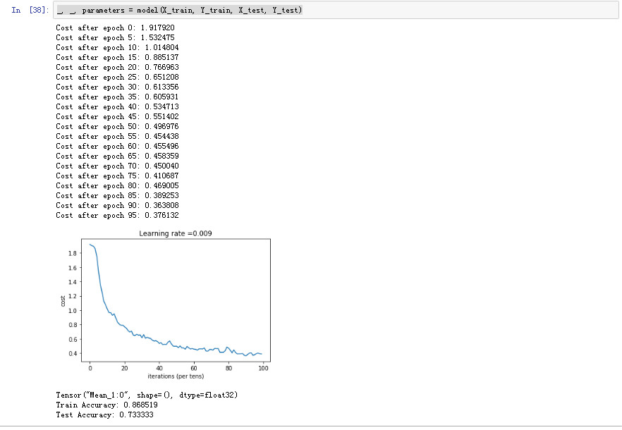
print ("Cost after epoch %i: %f" % (epoch, minibatch_cost))
if print_cost == True and epoch % 1 == 0:
costs.append(minibatch_cost)
# plot the cost
plt.plot(np.squeeze(costs))
plt.ylabel('cost')
plt.xlabel('iterations (per tens)')
plt.title("Learning rate =" + str(learning_rate))
plt.show()
# Calculate the correct predictions
predict_op = tf.argmax(Z3, 1) # Z3.shape=(m,6), 此處取每一個最大預測值最大位置的索引
correct_prediction = tf.equal(predict_op, tf.argmax(Y, 1)) #對比這兩個矩陣或者向量的相等的元素,如果是相等的那就返回True,反正返回False
# Calculate accuracy on the test set and the train set
accuracy = tf.reduce_mean(tf.cast(correct_prediction, "float")) # accuracy 是一個tensor
print(accuracy)
train_accuracy = accuracy.eval({X: X_train, Y: Y_train}) # PalceHolder
test_accuracy = accuracy.eval({X: X_test, Y: Y_test}) # .eval 執行計算圖
print("Train Accuracy:", train_accuracy)
print("Test Accuracy:", test_accuracy)
return train_accuracy, test_accuracy, parameters
X_train_orig , Y_train_orig , X_test_orig , Y_test_orig , classes = tf_utils.load_dataset()
Y_train = tf_utils.convert_to_one_hot(Y_train_orig, 6).T #convert_to_one_hot(Y, C)函數參見課程二第三周的2、programming assignments: 1.4 Using One Hot Encodeings
Y_test = tf_utils.convert_to_one_hot(Y_test_orig, 6).T
X_train = X_train_orig/255.
X_test = X_test_orig/255.
_, _, parameters = model(X_train, Y_train, X_test, Y_test,num_epochs=150)
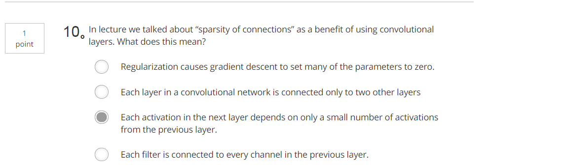
題目

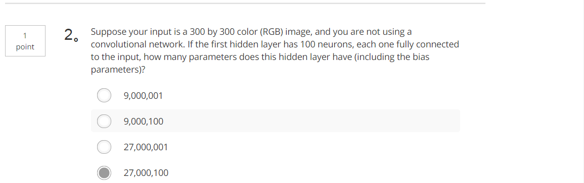 Tips:100×(300×300×3)+ 100=27000100
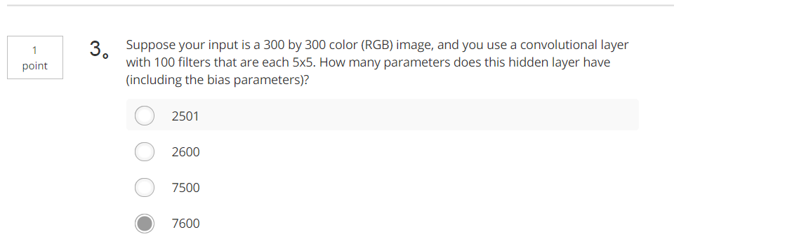 Tips:5×5×300+100=7600
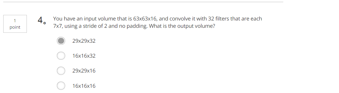 Tips:(63-7)/2+1=29
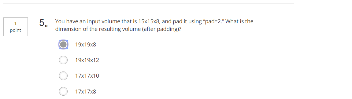 Tips:15+2×2=19
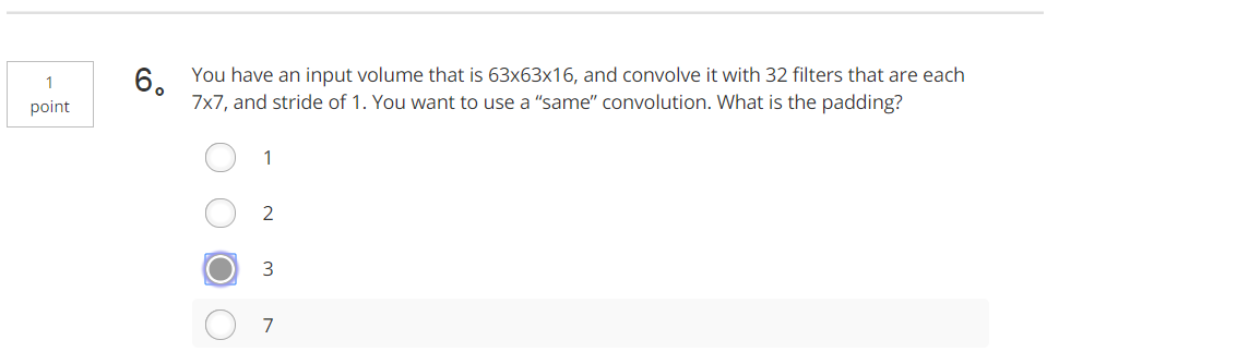 Tips:63+2p-7+1=63
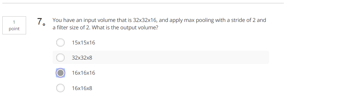 Tips:32/2
智能推薦
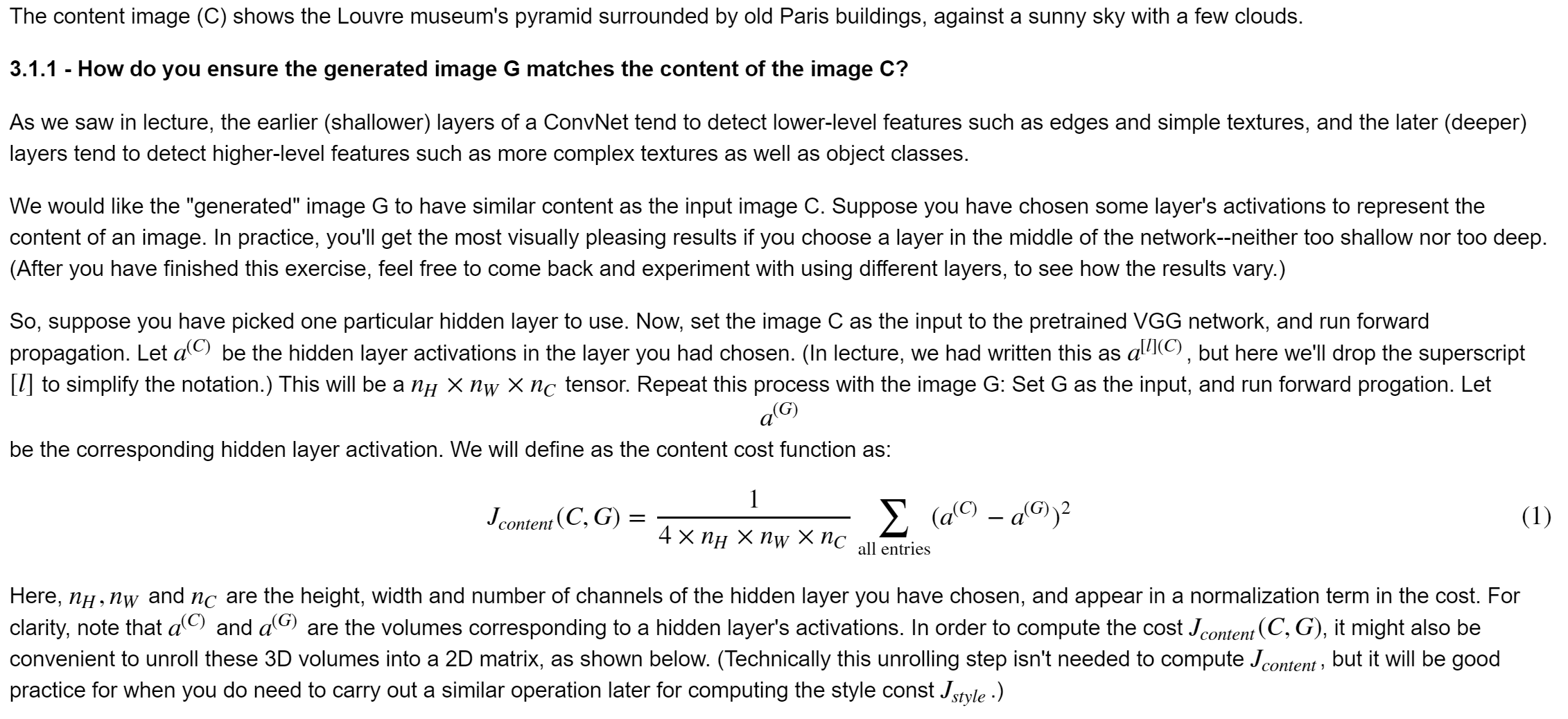
[深度學習] 第四課 Deep Learning & Art: Neural Style Transfer:編程練習-學習筆記
Deep Learning & Art: Neural Style Transfer Welcome to the second assignment of this week. In this assignment, you will learn about Neural Style Transfer. This algorithm was created by Gatys et al....
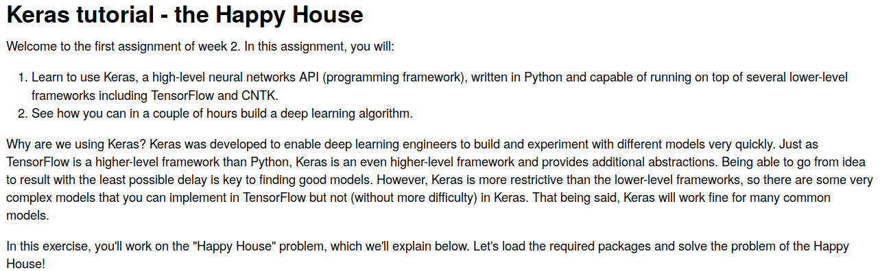
深度學習-卷積神經網絡 吳恩達第四課第二周作業1答案(Keras tutorial - the Happy House - to build a deep learning algorithm)
這里可顯示整個網絡的流程圖,若報錯提示無法輸出pydot,則參考博客 https://blog.csdn.net/Brianone/article/details/90111736...

吳恩達 Coursera Deep Learning 第五課 Sequence Models 第一周編程作業 2
Character level language model - Dinosaurus land¶ Welcome to Dinosaurus Island! 65 million years ago, dinosaurs existed, and in this assignment they are back. You are in charge of a special task....
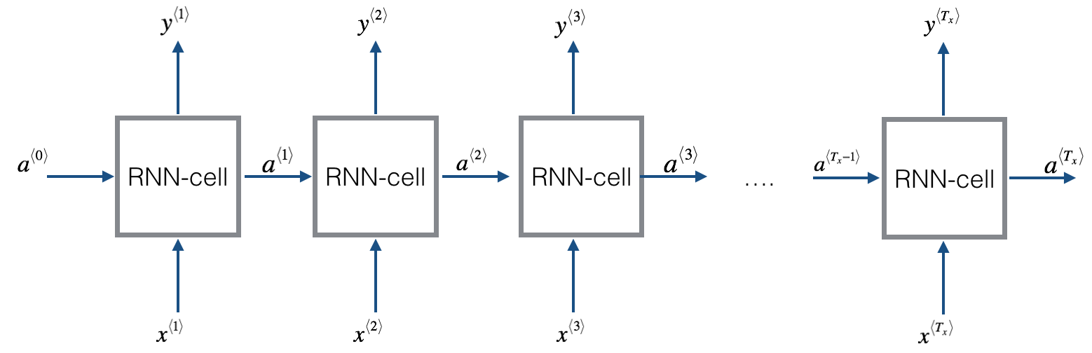
吳恩達 Coursera Deep Learning 第五課 Sequence Models 第一周編程作業 1(部分選做)
Building your Recurrent Neural Network - Step by Step Welcome to Course 5's first assignment! In this assignment, you will implement your first Recurrent Neural Network in numpy. Recurrent Neural Netw...
《深度學習——Andrew Ng》第一課第三周編程作業
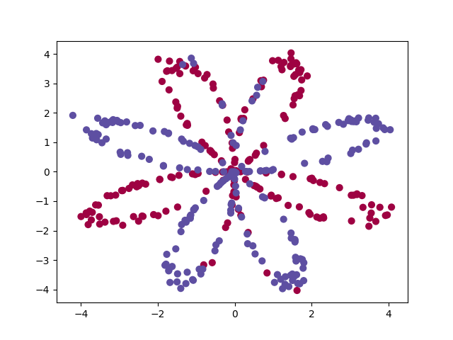
Planar data classification with one hidden layer You will see a big difference between this model and the one you implemented using logistic regression. You will learn how to: - Implement a 2-class cl...
猜你喜歡
deeplearning.ai 第四課第一周, 卷積神經網絡的tensorflow實現
1、載入需要模塊和函數: 2、載入數據及數據處理: 二、模型定義開始: 1、定義place_holder創造函數: 2、定義初始化函數: 3、定義前向傳播函數(此處到全連接層,并無**函數) 4、定義代價函數計算: 5、模型定義:模型中創建應按照如下步驟: create placeholders initialize parameters forward propagate compute the...


freemarker + ItextRender 根據模板生成PDF文件
1. 制作模板 2. 獲取模板,并將所獲取的數據加載生成html文件 2. 生成PDF文件 其中由兩個地方需要注意,都是關于獲取文件路徑的問題,由于項目部署的時候是打包成jar包形式,所以在開發過程中時直接安照傳統的獲取方法沒有一點文件,但是當打包后部署,總是出錯。于是參考網上文章,先將文件讀出來到項目的臨時目錄下,然后再按正常方式加載該臨時文件; 還有一個問題至今沒有解決,就是關于生成PDF文件...
電腦空間不夠了?教你一個小秒招快速清理 Docker 占用的磁盤空間!
Docker 很占用空間,每當我們運行容器、拉取鏡像、部署應用、構建自己的鏡像時,我們的磁盤空間會被大量占用。 如果你也被這個問題所困擾,咱們就一起看一下 Docker 是如何使用磁盤空間的,以及如何回收。 docker 占用的空間可以通過下面的命令查看: TYPE 列出了docker 使用磁盤的 4 種類型: Images:所有鏡像占用的空間,包括拉取下來的鏡像,和本地構建的。 Con...

requests實現全自動PPT模板
http://www.1ppt.com/moban/ 可以免費的下載PPT模板,當然如果要人工一個個下,還是挺麻煩的,我們可以利用requests輕松下載 訪問這個主頁,我們可以看到下面的樣式 點每一個PPT模板的圖片,我們可以進入到詳細的信息頁面,翻到下面,我們可以看到對應的下載地址 點擊這個下載的按鈕,我們便可以下載對應的PPT壓縮包 那我們就開始做吧 首先,查看網頁的源代碼,我們可以看到每一...