【Scikit-Learn】SVM示意圖
%matplotlib inline
import matplotlib.pyplot as plt
import numpy as np

class1 = np.array([[1, 1], [1, 3], [2, 1], [1, 2], [2, 2]])
class2 = np.array([[4, 4], [5, 5], [5, 4], [5, 3], [4, 5], [6, 4]])

plt.figure(figsize=(8, 6), dpi=144)

plt.title('Decision Boundary')

plt.xlim(0, 8)
plt.ylim(0, 6)
ax = plt.gca()                                  # gca 代表當前坐標軸,即 'get current axis'
ax.spines['right'].set_color('none')            # 隱藏坐標軸
ax.spines['top'].set_color('none')

plt.scatter(class1[:, 0], class1[:, 1], marker='o')
plt.scatter(class2[:, 0], class2[:, 1], marker='s')
plt.plot([1, 5], [5, 1], '-r')
plt.arrow(4, 4, -1, -1, shape='full', color='r')
plt.plot([3, 3], [0.5, 6], '--b')
plt.arrow(4, 4, -1, 0, shape='full', color='b', linestyle='--')
plt.annotate(r'margin 1',
             xy=(3.5, 4), xycoords='data',
             xytext=(3.1, 4.5), fontsize=10,
             arrowprops=dict(arrowstyle="->", connectionstyle="arc3,rad=.2"))
plt.annotate(r'margin 2',
             xy=(3.5, 3.5), xycoords='data',
             xytext=(4, 3.5), fontsize=10,
             arrowprops=dict(arrowstyle="->", connectionstyle="arc3,rad=.2"))
plt.annotate(r'support vector',
             xy=(4, 4), xycoords='data',
             xytext=(5, 4.5), fontsize=10,
             arrowprops=dict(arrowstyle="->", connectionstyle="arc3,rad=.2"))
plt.annotate(r'support vector',
             xy=(2, 2), xycoords='data',
             xytext=(0.5, 1.5), fontsize=10,
             arrowprops=dict(arrowstyle="->", connectionstyle="arc3,rad=.2"))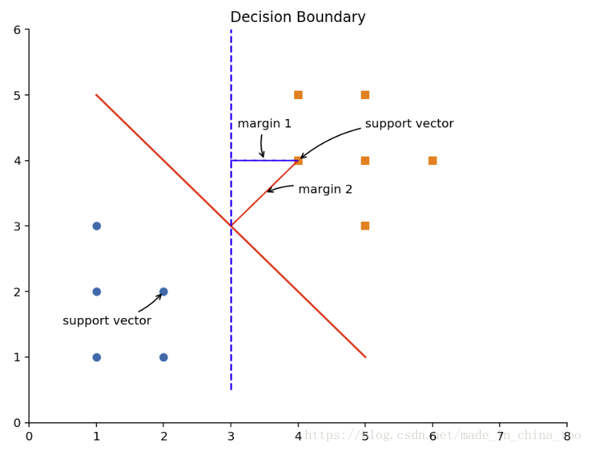
plt.figure(figsize=(8, 6), dpi=144)

plt.title('Support Vector Machine')

plt.xlim(0, 8)
plt.ylim(0, 6)
ax = plt.gca()                                  # gca 代表當前坐標軸,即 'get current axis'
ax.spines['right'].set_color('none')            # 隱藏坐標軸
ax.spines['top'].set_color('none')

plt.scatter(class1[:, 0], class1[:, 1], marker='o')
plt.scatter(class2[:, 0], class2[:, 1], marker='s')
plt.plot([1, 5], [5, 1], '-r')
plt.plot([0, 4], [4, 0], '--b', [2, 6], [6, 2], '--b')
plt.arrow(4, 4, -1, -1, shape='full', color='b')
plt.annotate(r'$w^T x + b = 0$',
             xy=(5, 1), xycoords='data',
             xytext=(6, 1), fontsize=10,
             arrowprops=dict(arrowstyle="->", connectionstyle="arc3,rad=.2"))
plt.annotate(r'$w^T x + b = 1$',
             xy=(6, 2), xycoords='data',
             xytext=(7, 2), fontsize=10,
             arrowprops=dict(arrowstyle="->", connectionstyle="arc3,rad=.2"))
plt.annotate(r'$w^T x + b = -1$',
             xy=(3.5, 0.5), xycoords='data',
             xytext=(4.5, 0.2), fontsize=10,
             arrowprops=dict(arrowstyle="->", connectionstyle="arc3,rad=.2"))
plt.annotate(r'd',
             xy=(3.5, 3.5), xycoords='data',
             xytext=(2, 4.5), fontsize=10,
             arrowprops=dict(arrowstyle="->", connectionstyle="arc3,rad=.2"))
plt.annotate(r'A',
             xy=(4, 4), xycoords='data',
             xytext=(5, 4.5), fontsize=10,
             arrowprops=dict(arrowstyle="->", connectionstyle="arc3,rad=.2"))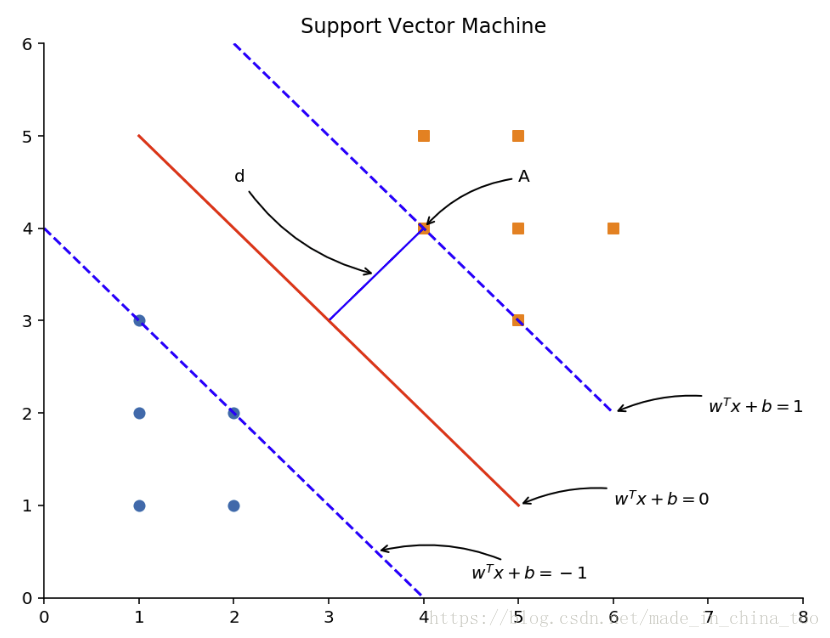
from sklearn.datasets import make_blobs

plt.figure(figsize=(13, 6), dpi=144)

# sub plot 1
plt.subplot(1, 2, 1)

X, y = make_blobs(n_samples=100,
                  n_features=2,
                  centers=[(1, 1), (2, 2)],
                  random_state=4,
                  shuffle=False,
                  cluster_std=0.4)

plt.title('Non-linear Separatable')

plt.xlim(0, 3)
plt.ylim(0, 3)
ax = plt.gca()                                  # gca 代表當前坐標軸,即 'get current axis'
ax.spines['right'].set_color('none')            # 隱藏坐標軸
ax.spines['top'].set_color('none')

plt.scatter(X[y==0][:, 0], X[y==0][:, 1], marker='o')
plt.scatter(X[y==1][:, 0], X[y==1][:, 1], marker='s')
plt.plot([0.5, 2.5], [2.5, 0.5], '-r')

# sub plot 2
plt.subplot(1, 2, 2)

class1 = np.array([[1, 1], [1, 3], [2, 1], [1, 2], [2, 2], [1.5, 1.5], [1.2, 1.7]])
class2 = np.array([[4, 4], [5, 5], [5, 4], [5, 3], [4, 5], [6, 4], [5.5, 3.5], [4.5, 4.5], [2, 1.5]])

plt.title('Slack Variable')

plt.xlim(0, 7)
plt.ylim(0, 7)
ax = plt.gca()                                  # gca 代表當前坐標軸,即 'get current axis'
ax.spines['right'].set_color('none')            # 隱藏坐標軸
ax.spines['top'].set_color('none')

plt.scatter(class1[:, 0], class1[:, 1], marker='o')
plt.scatter(class2[:, 0], class2[:, 1], marker='s')
plt.plot([1, 5], [5, 1], '-r')
plt.plot([0, 4], [4, 0], '--b', [2, 6], [6, 2], '--b')
plt.arrow(2, 1.5, 2.25, 2.25, shape='full', color='b')
plt.annotate(r'violate margin rule.',
             xy=(2, 1.5), xycoords='data',
             xytext=(0.2, 0.5), fontsize=10,
             arrowprops=dict(arrowstyle="->", connectionstyle="arc3,rad=.2"))
plt.annotate(r'normal sample. $\epsilon = 0$',
             xy=(4, 5), xycoords='data',
             xytext=(4.5, 5.5), fontsize=10,
             arrowprops=dict(arrowstyle="->", connectionstyle="arc3,rad=.2"))
plt.annotate(r'$\epsilon > 0$',
             xy=(3, 2.5), xycoords='data',
             xytext=(3, 1.5), fontsize=10,
             arrowprops=dict(arrowstyle="->", connectionstyle="arc3,rad=.2"))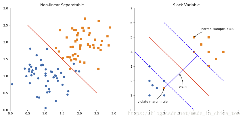
plt.figure(figsize=(8, 4), dpi=144)

plt.title('Cost')

plt.xlim(0, 4)
plt.ylim(0, 2)
plt.xlabel('$y^{(i)} (w^T x^{(i)} + b)$')
plt.ylabel('Cost')
ax = plt.gca()                                  # gca 代表當前坐標軸,即 'get current axis'
ax.spines['right'].set_color('none')            # 隱藏坐標軸
ax.spines['top'].set_color('none')

plt.plot([0, 1], [1.5, 0], '-r')
plt.plot([1, 3], [0.015, 0.015], '-r')
plt.annotate(r'$J_i = R \epsilon_i$ for $y^{(i)} (w^T x^{(i)} + b) \geq 1 - \epsilon_i$',
             xy=(0.7, 0.5), xycoords='data',
             xytext=(1, 1), fontsize=10,
             arrowprops=dict(arrowstyle="->", connectionstyle="arc3,rad=.2"))
plt.annotate(r'$J_i = 0$ for $y^{(i)} (w^T x^{(i)} + b) \geq 1$',
             xy=(1.5, 0), xycoords='data',
             xytext=(1.8, 0.2), fontsize=10,
             arrowprops=dict(arrowstyle="->", connectionstyle="arc3,rad=.2"))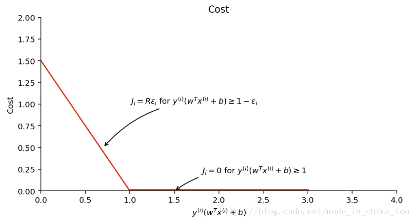
plt.figure(figsize=(13, 6), dpi=144)

class1 = np.array([[1, 1], [1, 2], [1, 3], [2, 1], [2, 2], [3, 2], [4, 1], [5, 1]])
class2 = np.array([[2.2, 4], [1.5, 5], [1.8, 4.6], [2.4, 5], [3.2, 5], [3.7, 4], [4.5, 4.5], [5.4, 3]])

# sub plot 1
plt.subplot(1, 2, 1)

plt.title('Non-linear Separatable in Low Dimension')

plt.xlim(0, 6)
plt.ylim(0, 6)
plt.yticks(())
plt.xlabel('X1')
ax = plt.gca()                                  # gca 代表當前坐標軸,即 'get current axis'
ax.spines['right'].set_color('none')            # 隱藏坐標軸
ax.spines['top'].set_color('none')
ax.spines['left'].set_color('none')

plt.scatter(class1[:, 0], np.zeros(class1[:, 0].shape[0]) + 0.05, marker='o')
plt.scatter(class2[:, 0], np.zeros(class2[:, 0].shape[0]) + 0.05, marker='s')

# sub plot 2
plt.subplot(1, 2, 2)

plt.title('Linear Separatable in High Dimension')

plt.xlim(0, 6)
plt.ylim(0, 6)
plt.xlabel('X1')
plt.ylabel('X2')
ax = plt.gca()                                  # gca 代表當前坐標軸,即 'get current axis'
ax.spines['right'].set_color('none')            # 隱藏坐標軸
ax.spines['top'].set_color('none')

plt.scatter(class1[:, 0], class1[:, 1], marker='o')
plt.scatter(class2[:, 0], class2[:, 1], marker='s')
plt.plot([1, 5], [3.8, 2], '-r')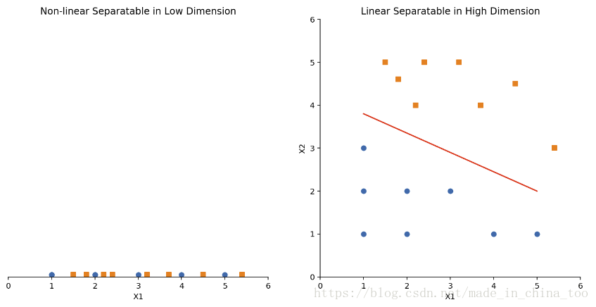
def gaussian_kernel(x, mean, sigma):
    return np.exp(- (x - mean)**2 / (2 * sigma**2))

x = np.linspace(0, 6, 500)
mean = 1
sigma1 = 0.1
sigma2 = 0.3

plt.figure(figsize=(10, 3), dpi=144)

# sub plot 1
plt.subplot(1, 2, 1)
plt.title('Gaussian for $\sigma={0}$'.format(sigma1))

plt.xlim(0, 2)
plt.ylim(0, 1.1)
ax = plt.gca()                                  # gca 代表當前坐標軸,即 'get current axis'
ax.spines['right'].set_color('none')            # 隱藏坐標軸
ax.spines['top'].set_color('none')

plt.plot(x, gaussian_kernel(x, mean, sigma1), 'r-')

# sub plot 2
plt.subplot(1, 2, 2)
plt.title('Gaussian for $\sigma={0}$'.format(sigma2))

plt.xlim(0, 2)
plt.ylim(0, 1.1)
ax = plt.gca()                                  # gca 代表當前坐標軸,即 'get current axis'
ax.spines['right'].set_color('none')            # 隱藏坐標軸
ax.spines['top'].set_color('none')

plt.plot(x, gaussian_kernel(x, mean, sigma2), 'r-')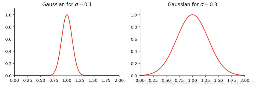
智能推薦
(10)Java中內存示意圖(其一)
程序是靜態的,存在于硬盤上,只有Load到內存中經過操作系統相關代碼調用后分配內存開始運行,Java代碼中又把內存分為4塊兒,如下圖:heap堆、stack棧、data segment、code segment。 八大基本類型與引用類型在內存中的區別: 八大基本類型在內存中只有一塊兒內存 而引用類型占兩塊兒內存 類和對象在...
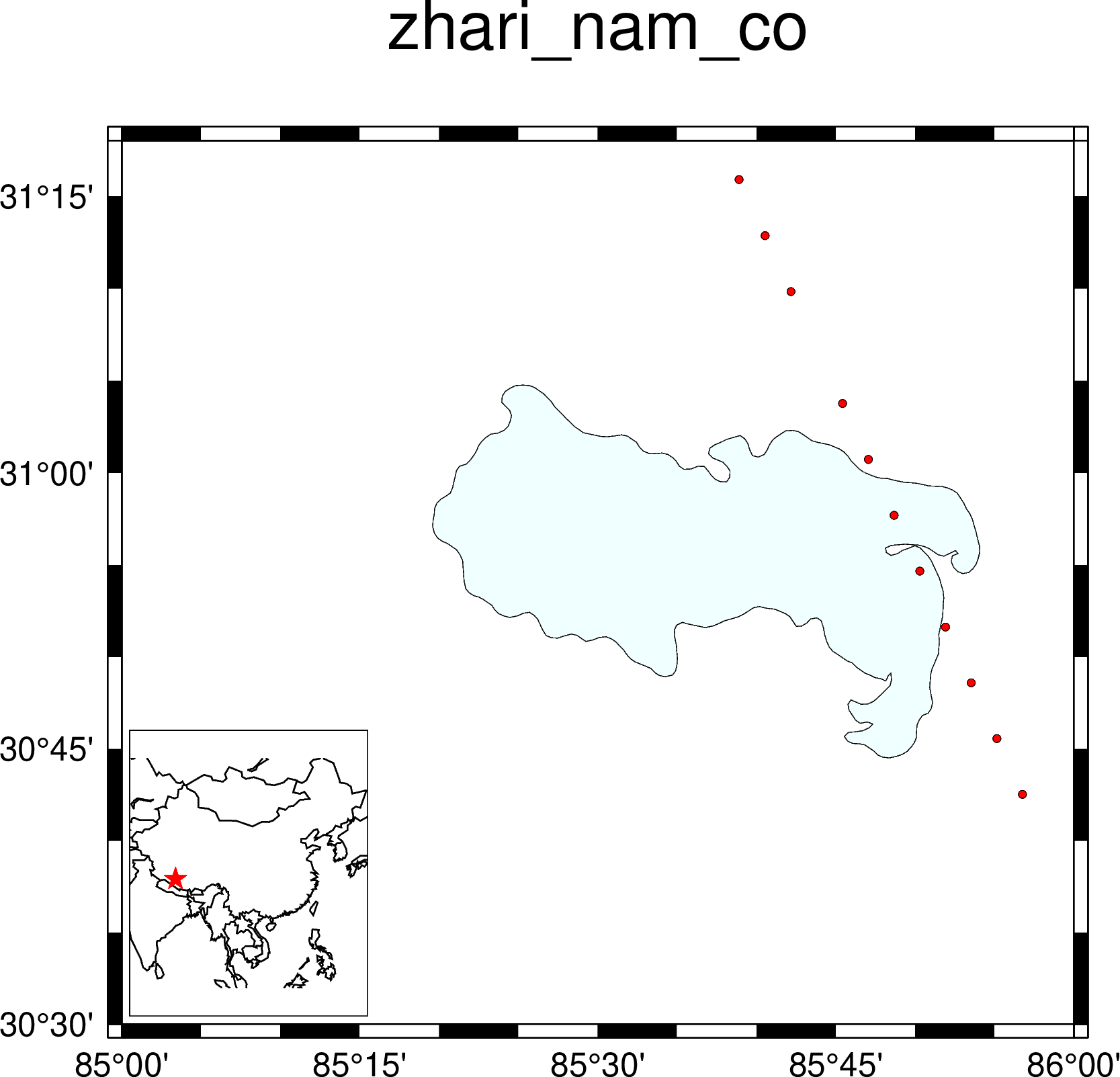
GMT繪制研究區示意圖(圖中圖)
. . 數語記吾學,以備不時之需,若遇同仁愿得賜教。 . . GMT繪制青藏高原某湖泊 ,GMT中文手冊104頁已有詳細介紹,僅做部分修改。 inset begin 定義了小圖的位置位于大圖左下角(-DjBL),小圖區域的寬度為 3 厘米,高度為 3.6 厘米(+w3c/3.6c),并且相對大圖左下角偏移 0.1 厘米(+o0.1c)。同時還設置了小圖區域的背景色為白色(+gwhite),并繪制了...
python程序構成、對象組成、內存示意圖
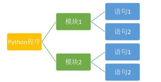
一、python程序的構成 1. Python 程序由模塊組成。一個模塊對應 python 源文件,一般后綴名是:.py。 2. 模塊由語句組成。運行 Python 程序時,按照模塊中語句的順序依次執行。 3. 語句是 Python 程序的構造單元,用于創建對象、變量賦值、調用函數、控制語句等。 4. python使用交互式環境,每次只能執行一條語句。 5. 代碼的組織和縮進:python通過縮進...
猜你喜歡


freemarker + ItextRender 根據模板生成PDF文件
1. 制作模板 2. 獲取模板,并將所獲取的數據加載生成html文件 2. 生成PDF文件 其中由兩個地方需要注意,都是關于獲取文件路徑的問題,由于項目部署的時候是打包成jar包形式,所以在開發過程中時直接安照傳統的獲取方法沒有一點文件,但是當打包后部署,總是出錯。于是參考網上文章,先將文件讀出來到項目的臨時目錄下,然后再按正常方式加載該臨時文件; 還有一個問題至今沒有解決,就是關于生成PDF文件...
電腦空間不夠了?教你一個小秒招快速清理 Docker 占用的磁盤空間!
Docker 很占用空間,每當我們運行容器、拉取鏡像、部署應用、構建自己的鏡像時,我們的磁盤空間會被大量占用。 如果你也被這個問題所困擾,咱們就一起看一下 Docker 是如何使用磁盤空間的,以及如何回收。 docker 占用的空間可以通過下面的命令查看: TYPE 列出了docker 使用磁盤的 4 種類型: Images:所有鏡像占用的空間,包括拉取下來的鏡像,和本地構建的。 Con...

requests實現全自動PPT模板
http://www.1ppt.com/moban/ 可以免費的下載PPT模板,當然如果要人工一個個下,還是挺麻煩的,我們可以利用requests輕松下載 訪問這個主頁,我們可以看到下面的樣式 點每一個PPT模板的圖片,我們可以進入到詳細的信息頁面,翻到下面,我們可以看到對應的下載地址 點擊這個下載的按鈕,我們便可以下載對應的PPT壓縮包 那我們就開始做吧 首先,查看網頁的源代碼,我們可以看到每一...