Andrew NG 機器學習 練習1-Linear Regression
在本次練習中,需要實現一個單變量的線性回歸。假設有一組歷史數據<城市人口,開店利潤>,現需要預測在哪個城市中開店利潤比較好?
歷史數據如下:第一列表示城市人口數,單位為萬人;第二列表示利潤,單位為10,000$
ex1data1.txt
6.1101,17.592
5.5277,9.1302
8.5186,13.662
7.0032,11.854
…
…
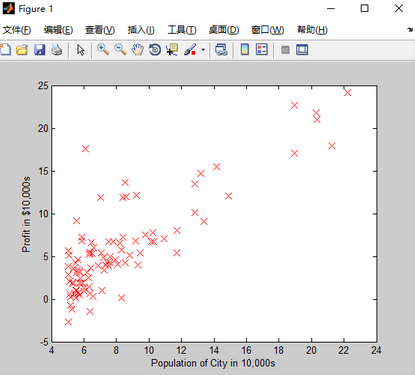
用Matlab畫出的圖形:首先加載數據,將data中的第一列數據保存到X中,將data中的所有行的第2列數據保存到y中
data = load('ex1data1.txt'); %讀取以逗號分隔的數據
X = data(:, 1); y = data(:, 2); %將第一列放在X向量中%將第二列放在y向量中
m = length(y); %測試數據的個數

% Plot Data
% Note: You have to complete the code in plotData.m
plotData(X, y);
plotData.m代碼如下:執行plot函數畫圖;xlabel、ylabel分別給X軸和Y軸標記提示信息。
function plotData(x, y)
%PLOTDATA Plots the data points x and y into a new figure
%   PLOTDATA(x,y) plots the data points and gives the figure axes labels of
%   population and profit.

figure; % open a new figure window

% ====================== YOUR CODE HERE ======================
% Instructions: Plot the training data into a figure using the
%               "figure" and "plot" commands. Set the axes labels using
%               the "xlabel" and "ylabel" commands. Assume the
%               population and revenue data have been passed in
%               as the x and y arguments of this function.
%
% Hint: You can use the 'rx' option with plot to have the markers
%       appear as red crosses. Furthermore, you can make the
%       markers larger by using plot(..., 'rx', 'MarkerSize', 10);

plot(x,y,'rx','MarkerSize',10); %plot the data, red顏色的X標記,標記的大小為 10
ylabel('Profit in $10,000s');
xlabel('Population of city in 10,000s');

% ============================================================

end
畫出來的圖形如下:
%% =================== Part 3: Cost and Gradient descent ===================
X = [ones(m, 1), data(:,1)]; % Add a column of ones to x
theta = zeros(2, 1); % initialize fitting parameters
% Some gradient descent settings
iterations = 1500;
alpha = 0.01; %learning rate
fprintf('\nTesting the cost function ...\n')
% compute and display initial cost
J = computeCost(X, y, theta);
fprintf('With theta = [0 ; 0]\nCost computed = %f\n', J);
fprintf('Expected cost value (approx) 32.07\n');
% further testing of the cost function
J = computeCost(X, y, [-1 ; 2]);
fprintf('\nWith theta = [-1 ; 2]\nCost computed = %f\n', J);
fprintf('Expected cost value (approx) 54.24\n');
fprintf('Program paused. Press enter to continue.\n');
pause;
fprintf('\nRunning Gradient Descent ...\n')
% run gradient descent
theta = gradientDescent(X, y, theta, alpha, iterations);
% print theta to screen
fprintf('Theta found by gradient descent:\n');
fprintf('%f\n', theta);
fprintf('Expected theta values (approx)\n');
fprintf(' -3.6303\n 1.1664\n\n');
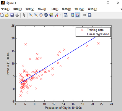
% Plot the linear fit
hold on; % keep previous plot visible
plot(X(:,2), X*theta, '-')
legend('Training data', 'Linear regression')
hold off % don't overlay any more plots on this figure
% Predict values for population sizes of 35,000 and 70,000
predict1 = [1, 3.5] *theta;
fprintf('For population = 35,000, we predict a profit of %f\n',...
predict1*10000);
predict2 = [1, 7] * theta;
fprintf('For population = 70,000, we predict a profit of %f\n',...
predict2*10000);
fprintf('Program paused. Press enter to continue.\n');
pause;function J = computeCost(X, y, theta)
%COMPUTECOST Compute cost for linear regression
% J = COMPUTECOST(X, y, theta) computes the cost of using theta as the
% parameter for linear regression to fit the data points in X and y
% Initialize some useful values
m = length(y); % number of training examples
% You need to return the following variables correctly
J = 0;
% ====================== YOUR CODE HERE ======================
% Instructions: Compute the cost of a particular choice of theta
% You should set J to the cost.
J=1/(2*m)*sum((X*theta-y).^2);
% =========================================================================
endfunction [theta, J_history] = gradientDescent(X, y, theta, alpha, num_iters)
%GRADIENTDESCENT Performs gradient descent to learn theta
% theta = GRADIENTDESCENT(X, y, theta, alpha, num_iters) updates theta by
% taking num_iters gradient steps with learning rate alpha
% Initialize some useful values
m = length(y); % number of training examples
J_history = zeros(num_iters, 1);
for iter = 1:num_iters
% ====================== YOUR CODE HERE ======================
% Instructions: Perform a single gradient step on the parameter vector
% theta.
%
% Hint: While debugging, it can be useful to print out the values
% of the cost function (computeCost) and gradient here.
%
theta=theta-(alpha/m)*X'*(X*theta-y);
% ============================================================
% Save the cost J in every iteration
J_history(iter) = computeCost(X, y, theta);
end
end求得的線性回歸模型如下圖:
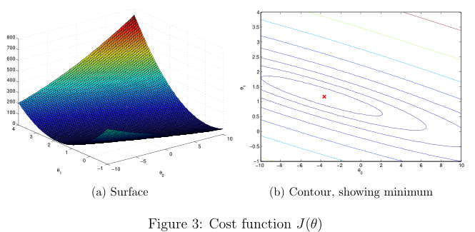
%% ============= Part 4: Visualizing J(theta_0, theta_1) =============
fprintf('Visualizing J(theta_0, theta_1) ...\n')

% Grid over which we will calculate J
theta0_vals = linspace(-10, 10, 100); %線性間隔向量,在-10和10之間100個點
theta1_vals = linspace(-1, 4, 100);

% initialize J_vals to a matrix of 0's
J_vals = zeros(length(theta0_vals), length(theta1_vals));

% Fill out J_vals
for i = 1:length(theta0_vals)
    for j = 1:length(theta1_vals)
      t = [theta0_vals(i); theta1_vals(j)];
      J_vals(i,j) = computeCost(X, y, t);
    end
end

% Because of the way meshgrids work in the surf command, we need to
% transpose J_vals before calling surf, or else the axes will be flipped
J_vals = J_vals';
% Surface plot
figure;
surf(theta0_vals, theta1_vals, J_vals)
xlabel('\theta_0'); ylabel('\theta_1');

% Contour plot
figure;
% Plot J_vals as 15 contours spaced logarithmically between 0.01 and 100
contour(theta0_vals, theta1_vals, J_vals, logspace(-2, 3, 20)) %繪制等高線,生成10的-2次方到10的3次方之間的按對數等分的n個元素的行向量
xlabel('\theta_0'); ylabel('\theta_1');
hold on;
plot(theta(1), theta(2), 'rx', 'MarkerSize', 10, 'LineWidth', 2);
多變量的線性回歸(Linear regression with multiple variables)
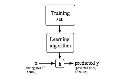
Suppose you are selling your house and you want to know what a good market price would be. One way to do this is to first collect information on recent houses sold and make a model of housing prices.
ex1data2.txt
The first column is the size of the house (in square feet),
the second column is the number of bedrooms,
and the third column is the price of the house.
2104,3,399900
1600,3,329900
2400,3,369000
1416,2,232000
…,…,…
…
標準化特征(Feature Normalization)
%% ================ Part 1: Feature Normalization ================

%% Clear and Close Figures
clear ; close all; clc

fprintf('Loading data ...\n');

%% Load Data
data = load('ex1data2.txt');
X = data(:, 1:2);
y = data(:, 3);
m = length(y);

% Print out some data points
fprintf('First 10 examples from the dataset: \n');
fprintf(' x = [%.0f %.0f], y = %.0f \n', [X(1:10,:) y(1:10,:)]');

fprintf('Program paused. Press enter to continue.\n');
pause;

% Scale features and set them to zero mean
fprintf('Normalizing Features ...\n');

[X,mu,sigma] = featureNormalize(X);


% Add intercept term to X
X = [ones(m, 1) X]
featureNormalize.m
function [X_norm, mu, sigma] = featureNormalize(X)
%FEATURENORMALIZE Normalizes the features in X
%   FEATURENORMALIZE(X) returns a normalized version of X where
%   the mean value of each feature is 0 and the standard deviation
%   is 1. This is often a good preprocessing step to do when
%   working with learning algorithms.

% You need to set these values correctly
X_norm = X;
mu = zeros(1, size(X, 2));
sigma = zeros(1, size(X, 2));

% ====================== YOUR CODE HERE ======================
% Instructions: First, for each feature dimension, compute the mean
%               of the feature and subtract it from the dataset,
%               storing the mean value in mu. Next, compute the
%               standard deviation of each feature and divide
%               each feature by it's standard deviation, storing
%               the standard deviation in sigma.
%
%               Note that X is a matrix where each column is a
%               feature and each row is an example. You need
%               to perform the normalization separately for
%               each feature.
%
% Hint: You might find the 'mean' and 'std' functions useful.
%

%方法1:按行求(提交有錯)
% mu=mean(X);
% sigma=[std(X(:,1)),std(X(:,2))];
% for i=1:size(X,1),
%     X_norm(i,:)=(X(i,:)-mu)./sigma;
% end;

%方法2:按列求
% for iter = 1:size(X, 2) %分兩列分別求
%     mu(1, iter) = mean(X(:, iter)); %第1或2列的均值
%     sigma(1, iter) = std(X(:, iter)); %第1或2列的標準差
%     X_norm(:, iter) = (X_norm(:, iter) - mu(1, iter)) ./ sigma(1, iter);

%方法3:向量化一起求
len = length(X);
mu = mean(X);
sigma = std(X);
X_norm = (X - ones(len, 1) * mu) ./ (ones(len, 1) * sigma);

% ============================================================

end
代價函數和梯度下降函數,可以復用單變量線性回歸實現,因為上述方法為向量化的矩陣操作,同樣適用于多變量
computeCostMulti.m
gradientDescentMulti.m
%% ================ Part 2: Gradient Descent ================

% ====================== YOUR CODE HERE ======================
% Instructions: We have provided you with the following starter
%               code that runs gradient descent with a particular
%               learning rate (alpha).
%
%               Your task is to first make sure that your functions -
%               computeCost and gradientDescent already work with
%               this starter code and support multiple variables.
%
%               After that, try running gradient descent with
%               different values of alpha and see which one gives
%               you the best result.
%
%               Finally, you should complete the code at the end
%               to predict the price of a 1650 sq-ft, 3 br house.
%
% Hint: By using the 'hold on' command, you can plot multiple
%       graphs on the same figure.
%
% Hint: At prediction, make sure you do the same feature normalization.
%

fprintf('Running gradient descent ...\n');

% Choose some alpha value
alpha = 0.01;
num_iters = 800;

% Init Theta and Run Gradient Descent
theta = zeros(3, 1);
[theta, J_history] = gradientDescentMulti(X, y, theta, alpha, num_iters);

% Plot the convergence graph
figure;
plot(1:numel(J_history), J_history, '-b', 'LineWidth', 2);
xlabel('Number of iterations');
ylabel('Cost J');

% Display gradient descent's result
fprintf('Theta computed from gradient descent: \n');
fprintf(' %f \n', theta);
fprintf('\n');

% Estimate the price of a 1650 sq-ft, 3 br house
% ====================== YOUR CODE HERE ======================
% Recall that the first column of X is all-ones. Thus, it does
% not need to be normalized.
X_test=[1650 3];
[X_test,mu,sigma] =featureNormalize2(X_test,mu,sigma);%使用樣本數據的均值,和標準差,進行歸一化
price = [1 X_test]*theta;

% ============================================================

fprintf(['Predicted price of a 1650 sq-ft, 3 br house ' ...
         '(using gradient descent):\n $%f\n'], price);

fprintf('Program paused. Press enter to continue.\n');
pause;

%% ================ Part 3: Normal Equations ================

fprintf('Solving with normal equations...\n');

% ====================== YOUR CODE HERE ======================
% Instructions: The following code computes the closed form
%               solution for linear regression using the normal
%               equations. You should complete the code in
%               normalEqn.m
%
%               After doing so, you should complete this code
%               to predict the price of a 1650 sq-ft, 3 br house.
%

%% Load Data
data = csvread('ex1data2.txt');
X = data(:, 1:2);
y = data(:, 3);
m = length(y);

% Add intercept term to X
X = [ones(m, 1) X];

% Calculate the parameters from the normal equation
theta = normalEqn(X, y);%使用正規方程的數據,不需要歸一化

% Display normal equation's result
fprintf('Theta computed from the normal equations: \n');
fprintf(' %f \n', theta);
fprintf('\n');


% Estimate the price of a 1650 sq-ft, 3 br house
% ====================== YOUR CODE HERE ======================
X_test=[1650 3];
price = [1 X_test]*theta;

% ============================================================

fprintf(['Predicted price of a 1650 sq-ft, 3 br house ' ...
         '(using normal equations):\n $%f\n'], price);
使用正規方程方法,求參數
normalEqn.m
function [theta] = normalEqn(X, y)
%NORMALEQN Computes the closed-form solution to linear regression
%   NORMALEQN(X,y) computes the closed-form solution to linear
%   regression using the normal equations.

theta = zeros(size(X, 2), 1);

% ====================== YOUR CODE HERE ======================
% Instructions: Complete the code to compute the closed form solution
%               to linear regression and put the result in theta.
%

% ---------------------- Sample Solution ----------------------
theta = pinv(X' * X) * X' * y

% ============================================================

end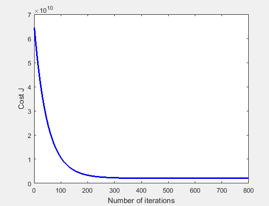
智能推薦
ML - Coursera Andrew Ng - Week1 & Week2 & Ex1 - Linear Regression - 筆記與代碼
Week 1和Week 2主要講解了機器學習中的一些基礎概念,并介紹了線性回歸算法(Linear Regression)。 機器學習主要分為三類: 監督學習(Supervised Learning):已知給定輸入的數據集的輸出結果。監督學習是學習輸入和輸出之間的映射關系。根據輸出值的類型監督學習問題可分為回歸(regression)問題和分類(classification)問題。如果輸出值是連續的...
Andrew Ng 機器學習筆記總結
本文由 CDFMLR 原創,收錄于個人主頁 https://clownote.github.io,并同時發布到 CSDN。本人不保證 CSDN 排版正確,敬請訪問 clownote 以獲得良好的閱讀體驗。 機器學習 Emmmm,這學期在 Coursera 學完了 Andrew Ng 的 Machine Learning 課程。我對這個課程一向是不以為意的,卻不小心報了個名,還手賤申請了個經濟援助,...
Andrew Ng機器學習筆記(五)
一、簡介 二、主要內容 Neural Networks Representation: Non-linear hypothesis: Neurons and the brain: Model representation: Examples and intuitions: Multi-class classification: Cost function: Backpropagation algo...
Andrew Ng機器學習筆記(三)
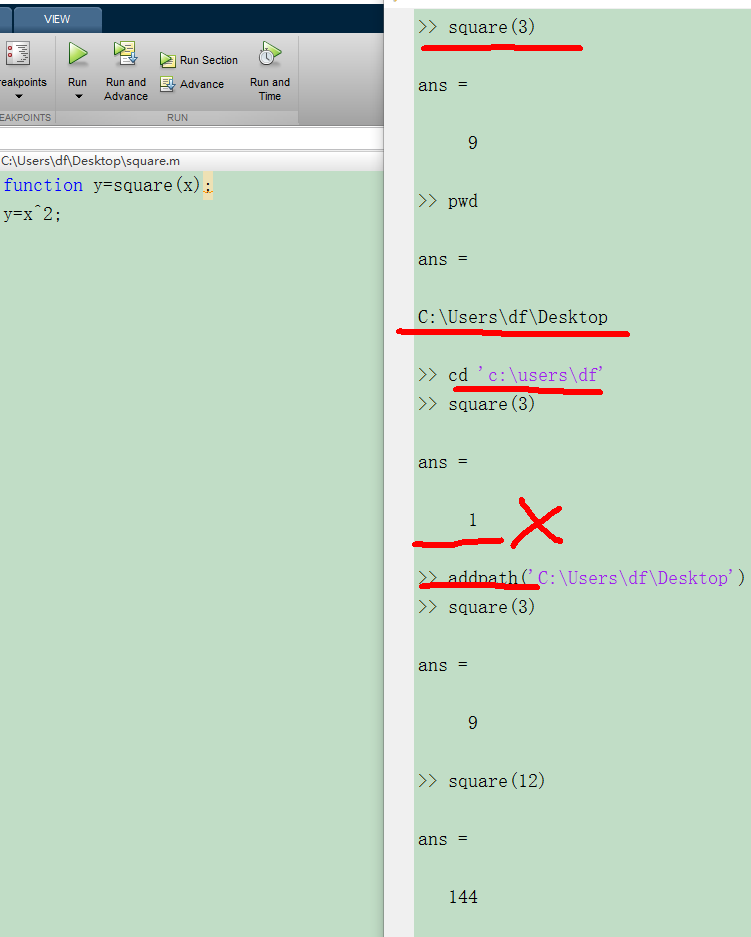
5.matlab教程 原始視頻使用的是Octave語言,與matlab很類似,這里用它代替。 函數路徑問題: 定義一個函數,square,求得是數值的平方。運行結果正確。輸入“pwd”,顯示當前的函數路徑。使用“cd”,修改路徑后,發現函數運行不能顯示正確結果。那么可以考慮,使用’addpath’命令,則函數可以正常運行。當然...

Machine Learning(Andrew Ng)ex2.logistic regression
Exam1 Exam2 Admitted 0 34.623660 78.024693 0 1 30.286711 43.894998 0 2 35.847409 72.902198 0 3 60.182599 86.308552 1 4 79.032736 75.344376 1 Exam1 Exam2 Admitted 0 34.623660 78.024693 0 1 30.286711 43...
猜你喜歡

【Machine Learning】【Andrew Ng】- notes(Week 3: Logistic Regression Model)
Cost Function We cannot use the same cost function that we use for linear regression because the Logistic Function will cause the output to be wavy, causing many local optima. In other words, it will ...
Andrew NG 機器學習 練習8-Anomaly Detection and Recommender Systems
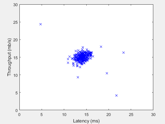
1 Anomaly detection 實現一個異常檢測算法檢測服務器的異常行為 特征是 每個服務器的 吞吐量(throughput)(mb/s) 和 相應延遲(ms) 采集 m=307 臺運行中的服務器的特征,{x(1),...,x(m)} 其中大部分是 normal 的服務器特征 你將使用 高斯模型 檢測數據集中的異常樣例 從 2D 數據集開始,以便可視化算法過程 在那個數據集中你將擬合一個高...
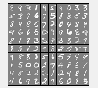
Andrew NG 機器學習 練習3-Multiclass Classification and Neural Networks
In this exercise, you will implement one-vs-all logistic regression and neural networks to recognize hand-written digits. 1 Multi-class Classification In the first part of the exercise, you will exten...


freemarker + ItextRender 根據模板生成PDF文件
1. 制作模板 2. 獲取模板,并將所獲取的數據加載生成html文件 2. 生成PDF文件 其中由兩個地方需要注意,都是關于獲取文件路徑的問題,由于項目部署的時候是打包成jar包形式,所以在開發過程中時直接安照傳統的獲取方法沒有一點文件,但是當打包后部署,總是出錯。于是參考網上文章,先將文件讀出來到項目的臨時目錄下,然后再按正常方式加載該臨時文件; 還有一個問題至今沒有解決,就是關于生成PDF文件...