Coursera | Andrew Ng (01-week-2-2.13)—向量化 Logistic 回歸
該系列僅在原課程基礎上部分知識點添加個人學習筆記,或相關推導補充等。如有錯誤,還請批評指教。在學習了 Andrew Ng 課程的基礎上,為了更方便的查閱復習,將其整理成文字。因本人一直在學習英語,所以該系列以英文為主,同時也建議讀者以英文為主,中文輔助,以便后期進階時,為學習相關領域的學術論文做鋪墊。- ZJ
轉載請注明作者和出處:ZJ 微信公眾號-「SelfImprovementLab」
知乎:https://zhuanlan.zhihu.com/c_147249273
CSDN:http://blog.csdn.net/JUNJUN_ZHAO/article/details/78931540
Vectorizing Logistic Regression 向量化 Logistic 回歸
(字幕來源:網易云課堂)
We have talked about how vectorization.lets you speed up your code significantly.In this video, we’ll talk about how you can vectorize the implementation of logistic regression,so they can process an entire training set,that is implement a single iteration of gradient descent with respect to an entire training set,without using even a single explicit for loop.I’m super excited about this technique,and when we talk about neural networks later and when we talk about neural networks later.Let’s get started. Let’s first examine the forward propagation steps of logistic regression.So, if you have m training examples,then to make a prediction on the first example,you need to compute that,compute z. I’m using this familiar formula,then compute the activations,you compute y hat in the first example.
我們已經討論過向量化,是如何顯著地加速你的代碼,在這次視頻中,我們將會談及向量化是如何實現在 logistic 回歸的上面的,這樣就能同時處理整個訓練集,來實現梯度下降法的一步迭代,針對整個訓練集的一步迭代,不需要使用任何顯式 for 循環,對于這一項技術,我特別興奮,并且當我們后面談及神經網絡時,也可以完全不用顯式 for 循環,那我們開始吧,我們先回顧,logistic 回歸的正向傳播步驟,如果你有 m 個訓練樣本,那么對第一個樣本進行預測,你需要這樣計算,計算出 z 運用這個熟悉的公式,然后計算**函數,計算在第一個樣本的 y帽 ()。
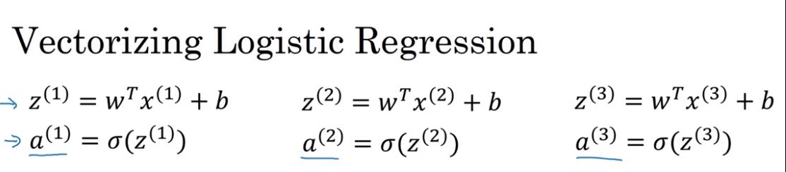
Then to make a prediction on the second training example,you need to compute that.Then, to make a prediction on the third example,you need to compute that, and so on.And you might need to do this m times,if you have M training examples.So, it turns out,that in order to carry out the forward propagation step,that is to compute these predictions on our m training examples,there is a way to do so,without needing an explicit for loop.
然后繼續去對第二個訓練樣本做一個預測,你需要這樣計算,然后去對第三個樣本做一個預測,你需要這樣計算,以此類推,你可能需要這樣做上 m 次,如果你有 m 個樣本,可以看出,為了執行正向傳播步驟,需要對 m 個訓練樣本 都計算出預測結果,但有一個辦法可以,不需要任何一個顯式的 for 循環。
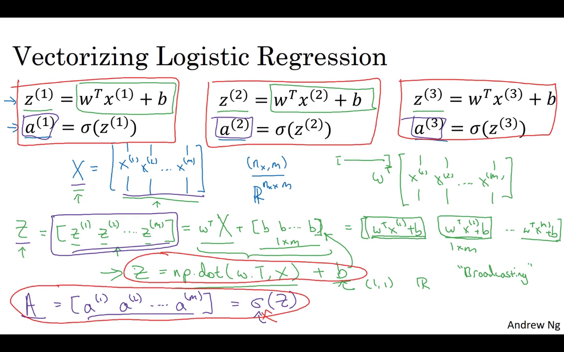
Let’s see how you can do it.First, remember that we defined a matrix capital X to be your training inputs,stacked together in different columns like this.So, this is a matrix,So, I’m writing this as a Python numpy shape,this just means that X is a n_x by m dimensional matrix.Now, the first thing I want to do is show how you can compute , , and so on,all in one step,in fact, with one line of code.
讓我們看看如何做到,首先記得我們曾定義過一個矩陣大寫 ,來作為你的訓練輸入,像這樣子在不同的列中堆疊在一起,這就是一個矩陣,這是一個的矩陣,我現在寫的是Python numpy形式,這只是意味 是一個的矩陣,現在我首先想要做的是 告訴你如何計算 ,以及 等等,全都在一個步驟中,事實上僅用了一行代碼。
So, I’m going to construct a 1 by M matrix,that’s really a row vector while I’m going to compute ,, and so on,down to ZM, all at the same time.It turns out that this can be expressed as W transpose to capital matrix X plus and then this vector B,B and so on.B, where this thing,this B, B, B, B, b thing is a 1 x m vector or 1 x m matrix or that is as a M dimensional row vector.
所以我要先構建一個 1 x m 的矩陣,實際上就是一個行向量 然后當我計算, 等等,一直到 都是在同一時間內,結果發現它可以表達成,w 的轉置 乘以大寫矩陣 加上這個向量 b,b b 等等,b 這個東西,這個 b b b b 這個東西就是一個1 x m的向量 或者,1 x m的矩陣 或者說是一個 m 維的行向量。
So hopefully there you are with matrix multiplication.You might see that W transpose X1, x2 and so on to XM,that W transpose can be a row vector.So this W transpose will be a row vector like that.And so this first term will evaluate to W transpose X1,W transpose X2 and so on, dot, dot, dot,W transpose XM, and then we add this second term B,B, B, and so on,you end up adding B to each element.So you end up with another 1xm vector.Well that’s the first element,that’s the second element and so on,and that’s the nth element.
希望你比較熟悉矩陣乘法,那么就會發現 W 轉置· 等等 一直到 ,這個 w 轉置可以是一個行向量,所以 w 轉置會是一個這樣的行向量,所以第一個項求的是 w 轉置乘 ,w 轉置乘 等等 點點點,w 轉置乘 然后我們加上第二項 b,b b 等等,最后是給每個元素加上 b,最后得到一個 1×m 向量,這是第一個元素,這是第二個元素等等,這是第 n 個元素 。
And if you refer to the definitions above,this first element is exactly the definition of .The second element is exactly the definition of and so on.So just as X was once obtained, when you took your training examples and stacked them next to each other, stacked them horizontally.I’m going to define capital Z to be this where you take the lowercase Z’s and stack them horizontally.So when you stack the lower case X’s corresponding to a different training examples,horizontally you get this variable capital X and the same way when you take these lowercase Z variables,and stack them horizontally,you get this variable capital Z.
如果你參考上面的定義,第一個元素恰恰是的定義,第二個元素恰恰是的定義 等等,是把所有訓練樣本堆疊起來得到的,一個挨著一個 橫向堆疊,我將會把大寫定義為這個 在這里,你用小寫 表示 橫向排在一起,所以當你將對應于不同訓練樣本的,小寫橫向堆疊起來時,你得到了這個變量 大寫,小寫變量也是同樣的處理,把它們橫向地堆疊起來,你就得到了這個變量大寫。
And it turns out, that in order to implement this,the numpy command is capital Z equals NP dot w dot T,that’s w transpose X and then plus b.Now there is a subtlety in Python,which is at here b is a real number or if you want to say you know 1x1 matrix,is just a normal real number.But, when you add this vector to this real number,Python automatically takes this real number B and expands it out to this 1XM row vector.So in case this operation seems a little bit mysterious,this is called broadcasting in Python,and you don’t have to worry about it for now,we’ll talk about it some more in the next video.
結果發現 為了計算這個,numpy 的指令為大寫 Z = np.dot(w.T ..,那是w的轉置 .. ,x) + b,這里有個 Python 巧妙的地方,在這個地方b是一個實數,或者你可以說是 1×1 的矩陣,就是一個普通的實數,但是 當你把向量加上這個實數時,Python 會自動的把實數 b,擴展成一個 1×m 的行向量,所以這個操作看上去有一點神秘,在 Python 中這叫做廣播( broadcasting ),目前你不用對此感到顧慮,我們會在下一節視頻中更多地談及它 .
But the takeaway is that with just one line of code,with this line of code,you can calculate capital Z and capital Z is going to be a 1XM matrix that contains all of the lower cases Z’s.Lowercase through lower case ZM.So that was Z, how about these values a.What we like to do next is find a way to compute ,and so on to ,all at the same time,and just as stacking lowercase X’s resulted in capital X and stacking horizontally lowercase Z’s resulted in capital Z,stacking lower case A, is going to result in a new variable,which we are going to define as capital A.
再說回來只要用一行的代碼,運用這行代碼,你可以計算大寫 Z,而大寫 Z 是一個 1×m 的矩陣,包含所有的小寫 z,小寫一直到小寫 ,這就是 Z 那么變量 a 是怎樣的呢,我們接下去要做的,是找到一個辦法來計算 , 等等一直到 ,都在同一時間完成,就像把小 x 堆疊起來形成 X 一樣,將小 z 橫向堆疊成大 Z,堆疊小寫 a 就會形成一個新的變量,我們把它定義為大寫 A。
And in the program assignment,you see how to implement a vector valued function,so that the function,inputs this capital Z as a variable and very efficiently outputs capital A.So you see the details of that in the programming assignment.So just to recap,what we’ve seen on this slide is that instead of needing to loop over M training examples to compute lowercase z and lowercase a,one of the time, you can implement this one line of code,to compute all these Z’s at the same time.
在編程作業中,你能看到如何對一個向量進行 函數操作,所以 函數,把大寫 Z 當做一個變量進行輸入,然后非常高效的輸出大寫 A,你仔細看看編程作業里的細節,總的來說,我們在這張幻燈片所看到的是 不需要 for 循環,就可以從 m 個訓練樣本 一次性計算出小寫 z 和小寫 a ,而你運行這些只需要一行代碼,在同一時間計算所有的 z。
And then, this one line of code,with appropriate implementation of lowercase Sigma to compute all the lowercase A’s all at the same time.So this is how you implement a vectorize implementation of the forward propagation for all M training examples at the same time.So to summarize, you’ve just seen how you can use vectorization to very efficiently compute all of the activations,all the lowercase a’s at the same time.Next, it turns out, you can also use vectorization very efficiently to compute the backward propagation,to compute the gradients.Let’s see how you can do that, in the next video.
這一行的代碼,實現的是,用小寫 sigma 同時計算所有小寫 a,所以這就是,正向傳播一步迭代的向量化實現,同時處理所有 m 個訓練樣本,概括一下 你剛剛看到如何使用向量化,高效計算**函數,同時輸出所有小 a,接下來 你會發現同樣可以用向量化,來高效地計算反向傳播,并以此來計算梯度,我們在下一次視頻中將看到它如何實現。
重點總結:
所有 m 個樣本的線性輸出 可以用矩陣表示:
Z = np.dot(w.T,X) + b
A = sigmoid(Z)
邏輯回歸梯度下降輸出向量化
對于個樣本,維度為,表示為:
db可以表示為:
db = 1/m * np.sum(dZ)- dw可表示為:
dw = 1/m*np.dot(X,dZ.T)參考文獻:
[1]. 大樹先生.吳恩達Coursera深度學習課程 DeepLearning.ai 提煉筆記(1-2)– 神經網絡基礎
PS: 歡迎掃碼關注公眾號:「SelfImprovementLab」!專注「深度學習」,「機器學習」,「人工智能」。以及 「早起」,「閱讀」,「運動」,「英語 」「其他」不定期建群 打卡互助活動。

智能推薦
斯坦福Andrew Ng---機器學習筆記(二):Logistic Regression(邏輯回歸)
轉載自:https://blog.csdn.net/xiaocainiaodeboke/article/details/50371986 內容提要 這篇博客的主要內容有: - 介紹欠擬合和過擬合的概念 - 從概率的角度解釋上一篇博客中評價函數J(θ)” role=”presentation” style=”position: r...
Andrew NG 機器學習 筆記-week3-邏輯回歸
一、分類和表示(Classification and Representation) 1.1 分類問題(Classification) 在分類問題中,你要預測的變量 y 是離散的值,我們將學習一種叫做邏輯回歸 (Logistic Regression) 的算法,這是目前最流行使用最廣泛的一種學習算法。 在分類問題中,我們嘗試預測的是結果是否屬于某一個類(例如正確或錯誤)。分類問題的例子有:判斷一封...
Coursera | Andrew Ng (02-week3)—超參數調試 Batch 正則化和程序框架
在吳恩達深度學習視頻以及大樹先生的博客提煉筆記基礎上添加個人理解,原大樹先生博客可查看該鏈接地址大樹先生的博客- ZJ Coursera 課程 |deeplearning.ai |網易云課堂 CSDN:http://blog.csdn.net/JUNJUN_ZHAO/article/details/79497132 3.1 Tuning process (調參處理) 早一代的機器學習算法中,超參數...
Coursera | Andrew Ng (02-week-1-1.11)—神經網絡的權重初始化
該系列僅在原課程基礎上部分知識點添加個人學習筆記,或相關推導補充等。如有錯誤,還請批評指教。在學習了 Andrew Ng 課程的基礎上,為了更方便的查閱復習,將其整理成文字。因本人一直在學習英語,所以該系列以英文為主,同時也建議讀者以英文為主,中文輔助,以便后期進階時,為學習相關領域的學術論文做鋪墊。- ZJ Coursera 課程 |deeplearning.ai |網易云課堂 轉載請注明作者和...
Coursera | Andrew Ng (02-week-1-1.6)—Dropout 正則化
該系列僅在原課程基礎上部分知識點添加個人學習筆記,或相關推導補充等。如有錯誤,還請批評指教。在學習了 Andrew Ng 課程的基礎上,為了更方便的查閱復習,將其整理成文字。因本人一直在學習英語,所以該系列以英文為主,同時也建議讀者以英文為主,中文輔助,以便后期進階時,為學習相關領域的學術論文做鋪墊。- ZJ Coursera 課程 |deeplearning.ai |網易云課堂 轉載請注明作者和...
猜你喜歡
Coursera | Andrew Ng (02-week3-3.2)—為超參數選擇合適的范圍
該系列僅在原課程基礎上部分知識點添加個人學習筆記,或相關推導補充等。如有錯誤,還請批評指教。在學習了 Andrew Ng 課程的基礎上,為了更方便的查閱復習,將其整理成文字。因本人一直在學習英語,所以該系列以英文為主,同時也建議讀者以英文為主,中文輔助,以便后期進階時,為學習相關領域的學術論文做鋪墊。- ZJ Coursera 課程 |deeplearning.ai |網易云課堂 轉載請注明作者和...
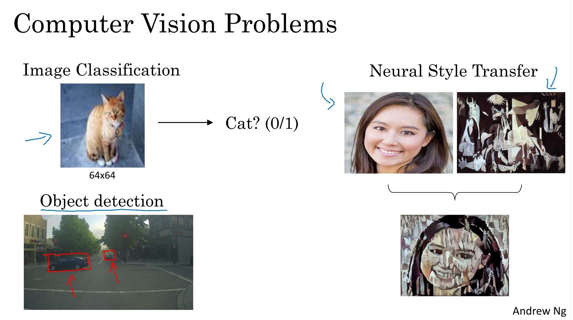
Coursera | Andrew Ng (04-week1)—卷積神經網絡
在吳恩達深度學習視頻以及大樹先生的博客提煉筆記基礎上添加個人理解,原大樹先生博客可查看該鏈接地址大樹先生的博客- ZJ Coursera 課程 |deeplearning.ai |網易云課堂 CSDN:http://blog.csdn.net/junjun_zhao/article/details/79190634 Convolutional Neural Networks (卷積神經網絡) We...
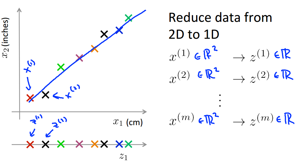
Coursera 機器學習(by Andrew Ng)課程學習筆記 Week 8(二)——降維
此系列為 Coursera 網站機器學習課程個人學習筆記(僅供參考) 課程網址:https://www.coursera.org/learn/machine-learning 參考資料:http://blog.csdn.net/MajorDong100/article/details/51104784 一、降維的作用 1.1 數據壓縮 數據壓縮(Data Compression)不僅能減少數據的存...
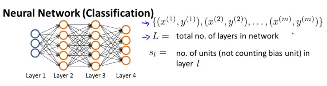
Coursera 機器學習(by Andrew Ng)課程學習筆記 Week 5——神經網絡(二)
此系列為 Coursera 網站機器學習課程個人學習筆記(僅供參考) 課程網址:https://www.coursera.org/learn/machine-learning 參考資料:http://blog.csdn.net/SCUT_Arucee/article/details/50176159 一、神經網絡的代價函數 1.1 神經網絡的模型參數 假設我們有下圖這樣的神經網絡: 我們定義以下符...
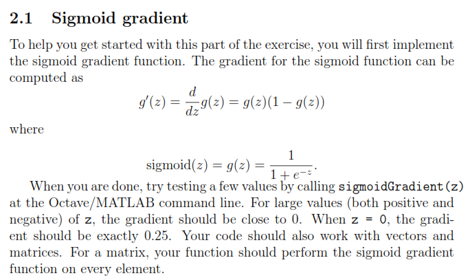
Andrew Ng coursera上的《機器學習》ex4
Andrew Ng coursera上的《機器學習》ex4 按照課程所給的ex4的文檔要求,ex4要求完成以下幾個計算過程的代碼編寫: exerciseName description sigmoidGradient.m compute the grident of the sigmoid function randInitializedWeights.m randomly initialize ...