Machine Learning(Andrew Ng）ex1.linear regression

Linear Regression

import tensorflow as tf
import pandas as pd
import matplotlib.pyplot as plt
import numpy as np
from mpl_toolkits.mplot3d import Axes3D

path='ex1data1.txt'
data=pd.read_csv(path,header=None,names=['Population','Profit'])
data.head()

	Population	Profit
0	6.1101	17.5920
1	5.5277	9.1302
2	8.5186	13.6620
3	7.0032	11.8540
4	5.8598	6.8233

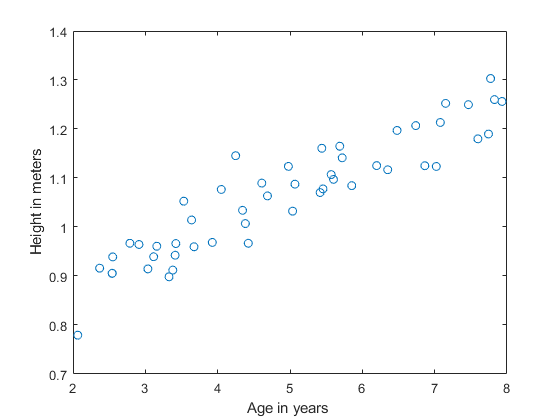
data.plot(kind='scatter',x='Population',y='Profit',figsize=(12,8))
plt.show()

在這里插入圖片描述

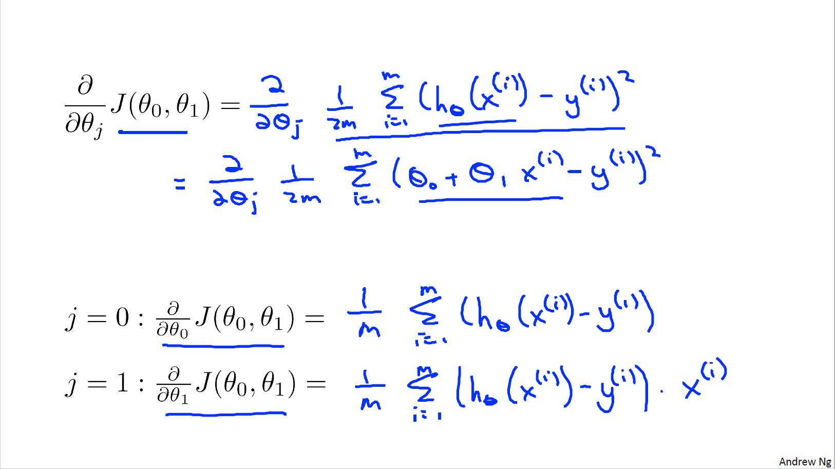
def computeCost(X, y, theta):
   J= np.sum(np.power(((X * theta.T) - y), 2))*(1/(2 * len(X)))
   return J

data.insert(0, 'Ones', 1)

cols = data.shape[1]
X = data.iloc[:,0:cols-1]
y = data.iloc[:,cols-1:cols]

X.head()

	Ones	Population
0	1	6.1101
1	1	5.5277
2	1	8.5186
3	1	7.0032
4	1	5.8598

y.head()

	Profit
0	17.5920
1	9.1302
2	13.6620
3	11.8540
4	6.8233

X = np.matrix(X.values)
y = np.matrix(y.values)
theta = np.matrix(np.array([0,0]))

theta

matrix([[0, 0]])

computeCost(X,y,theta)

32.072733877455676

$\theta_{j} :=\theta_{j}-\alpha \frac{1}{m} \sum_{i=1}^{m}\left(h_{\theta}\left(x^{(i)}\right)-y^{(i)}\right) x_{j}^{(i)},(j=0,1)$

theta.shape[1]

def gradientDescent(x,y,theta,alpha,iterations):
    temp=np.matrix(np.zeros(theta.shape[1]))#單變量x只有一個
    parameters=int(theta.shape[1])#theta的個數，ravel函數轉化成一列數組
    cost=[]
    #theta_0_history=[]
    #teeta_1_history=[]
    for i in range(iterations):
        error=(x*theta.T)-y
        for j in range(parameters):
            term=np.multiply(error,x[:,j])
            temp[0,j]=theta[0,j]-((alpha/len(x))*np.sum(term))
        theta=temp
        cost.append(computeCost(x,y,theta))
        #theta_0_history.append(temp[0,0])
        #theta_1_history.append(temp[0,1])
    return theta,cost

alpha=0.01
iters=1000

theta_new,cost=gradientDescent(X,y,theta,alpha,iters)

computeCost(X,y,theta_new)

4.515955503078912

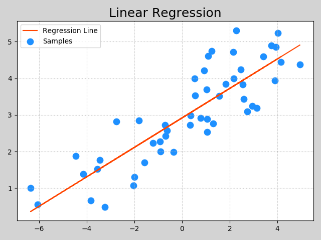
x=np.linspace(data.Population.min(),data.Population.max(),100)
f=theta_new[0,0]+theta_new[0,1]*x
fig,ax=plt.subplots(figsize=(12,8))
ax.plot(x,f,'y',label='Prediction')
ax.scatter(data.Population,data.Profit,marker='^',label='Trainning Data')
ax.set_xlabel('Population')
ax.set_ylabel('Profit')
ax.set_title('Predicted Profit vs. Population Size')
plt.show()

在這里插入圖片描述

matrix([[ 1.    ,  6.1101],
        [ 1.    ,  5.5277],
        [ 1.    ,  8.5186],
        [ 1.    ,  7.0032],
        [ 1.    ,  5.8598],
        [ 1.    ,  8.3829],
        [ 1.    ,  7.4764],
        [ 1.    ,  8.5781],
        [ 1.    ,  6.4862],
        [ 1.    ,  5.0546],
        [ 1.    ,  5.7107],
        [ 1.    , 14.164 ],
        [ 1.    ,  5.734 ],
        [ 1.    ,  8.4084],
        [ 1.    ,  5.6407],
        [ 1.    ,  5.3794],
        [ 1.    ,  6.3654],
        [ 1.    ,  5.1301],
        [ 1.    ,  6.4296],
        [ 1.    ,  7.0708],
        [ 1.    ,  6.1891],
        [ 1.    , 20.27  ],
        [ 1.    ,  5.4901],
        [ 1.    ,  6.3261],
        [ 1.    ,  5.5649],
        [ 1.    , 18.945 ],
        [ 1.    , 12.828 ],
        [ 1.    , 10.957 ],
        [ 1.    , 13.176 ],
        [ 1.    , 22.203 ],
        [ 1.    ,  5.2524],
        [ 1.    ,  6.5894],
        [ 1.    ,  9.2482],
        [ 1.    ,  5.8918],
        [ 1.    ,  8.2111],
        [ 1.    ,  7.9334],
        [ 1.    ,  8.0959],
        [ 1.    ,  5.6063],
        [ 1.    , 12.836 ],
        [ 1.    ,  6.3534],
        [ 1.    ,  5.4069],
        [ 1.    ,  6.8825],
        [ 1.    , 11.708 ],
        [ 1.    ,  5.7737],
        [ 1.    ,  7.8247],
        [ 1.    ,  7.0931],
        [ 1.    ,  5.0702],
        [ 1.    ,  5.8014],
        [ 1.    , 11.7   ],
        [ 1.    ,  5.5416],
        [ 1.    ,  7.5402],
        [ 1.    ,  5.3077],
        [ 1.    ,  7.4239],
        [ 1.    ,  7.6031],
        [ 1.    ,  6.3328],
        [ 1.    ,  6.3589],
        [ 1.    ,  6.2742],
        [ 1.    ,  5.6397],
        [ 1.    ,  9.3102],
        [ 1.    ,  9.4536],
        [ 1.    ,  8.8254],
        [ 1.    ,  5.1793],
        [ 1.    , 21.279 ],
        [ 1.    , 14.908 ],
        [ 1.    , 18.959 ],
        [ 1.    ,  7.2182],
        [ 1.    ,  8.2951],
        [ 1.    , 10.236 ],
        [ 1.    ,  5.4994],
        [ 1.    , 20.341 ],
        [ 1.    , 10.136 ],
        [ 1.    ,  7.3345],
        [ 1.    ,  6.0062],
        [ 1.    ,  7.2259],
        [ 1.    ,  5.0269],
        [ 1.    ,  6.5479],
        [ 1.    ,  7.5386],
        [ 1.    ,  5.0365],
        [ 1.    , 10.274 ],
        [ 1.    ,  5.1077],
        [ 1.    ,  5.7292],
        [ 1.    ,  5.1884],
        [ 1.    ,  6.3557],
        [ 1.    ,  9.7687],
        [ 1.    ,  6.5159],
        [ 1.    ,  8.5172],
        [ 1.    ,  9.1802],
        [ 1.    ,  6.002 ],
        [ 1.    ,  5.5204],
        [ 1.    ,  5.0594],
        [ 1.    ,  5.7077],
        [ 1.    ,  7.6366],
        [ 1.    ,  5.8707],
        [ 1.    ,  5.3054],
        [ 1.    ,  8.2934],
        [ 1.    , 13.394 ],
        [ 1.    ,  5.4369]])

fig=plt.figure(dpi=500)
ax = Axes3D(fig)
theta_0=np.linspace(-10,10,100)
theta_1=np.linspace(-1,4,100)
cos=np.arange(10000).reshape(100,100)
#t=np.matrix([theta_0,theta_1])
theta_0,theta_1=np.meshgrid(theta_0,theta_1)
for i in range(100):
    for j in range(100):
        t=np.matrix([theta_0[i],theta_1[j]])
        cos[i,j]=computeCost(X,y,t.T)
        
ax.plot_surface(theta_0,theta_1,cos,rstride=1,cstride=1,cmap=plt.get_cmap('rainbow'))
plt.show()

在這里插入圖片描述

fig, ax = plt.subplots(figsize=(12,8))
ax.plot(np.arange(iters),cost,'r')
ax.set_ylabel('Cost')
ax.set_title('Error vs. Training Epoch')
plt.show()

在這里插入圖片描述

Linear regression with multiple variables

path =  'ex1data2.txt'
data2 = pd.read_csv(path, header=None, names=['Size', 'Bedrooms', 'Price'])
data2.head()

	Size	Bedrooms	Price
0	2104	3	399900
1	1600	3	329900
2	2400	3	369000
3	1416	2	232000
4	3000	4	539900

data2 = (data2 - data2.mean()) / data2.std()
data2.head()

	Size	Bedrooms	Price
0	0.130010	-0.223675	0.475747
1	-0.504190	-0.223675	-0.084074
2	0.502476	-0.223675	0.228626
3	-0.735723	-1.537767	-0.867025
4	1.257476	1.090417	1.595389

data2.insert(0, 'Ones', 1)
data2.head()

	Ones	Size	Bedrooms	Price
0	1	0.130010	-0.223675	0.475747
1	1	-0.504190	-0.223675	-0.084074
2	1	0.502476	-0.223675	0.228626
3	1	-0.735723	-1.537767	-0.867025
4	1	1.257476	1.090417	1.595389

cols = data2.shape[1]
X2 = data2.iloc[:,0:cols-1]
y2 = data2.iloc[:,cols-1:cols]



# convert to matrices and initialize theta
X2 = np.matrix(X2.values)
y2 = np.matrix(y2.values)
theta2 = np.matrix(np.array([0,0,0]))
print(X2)
# perform linear regression on the data set
g2, cost2 = gradientDescent(X2, y2, theta2, alpha, iters)

# get the cost (error) of the model
computeCost(X2, y2, g2)

[[ 1.00000000e+00  1.30009869e-01 -2.23675187e-01]
 [ 1.00000000e+00 -5.04189838e-01 -2.23675187e-01]
 [ 1.00000000e+00  5.02476364e-01 -2.23675187e-01]
 [ 1.00000000e+00 -7.35723065e-01 -1.53776691e+00]
 [ 1.00000000e+00  1.25747602e+00  1.09041654e+00]
 [ 1.00000000e+00 -1.97317285e-02  1.09041654e+00]
 [ 1.00000000e+00 -5.87239800e-01 -2.23675187e-01]
 [ 1.00000000e+00 -7.21881404e-01 -2.23675187e-01]
 [ 1.00000000e+00 -7.81023044e-01 -2.23675187e-01]
 [ 1.00000000e+00 -6.37573110e-01 -2.23675187e-01]
 [ 1.00000000e+00 -7.63567023e-02  1.09041654e+00]
 [ 1.00000000e+00 -8.56737193e-04 -2.23675187e-01]
 [ 1.00000000e+00 -1.39273340e-01 -2.23675187e-01]
 [ 1.00000000e+00  3.11729182e+00  2.40450826e+00]
 [ 1.00000000e+00 -9.21956312e-01 -2.23675187e-01]
 [ 1.00000000e+00  3.76643089e-01  1.09041654e+00]
 [ 1.00000000e+00 -8.56523009e-01 -1.53776691e+00]
 [ 1.00000000e+00 -9.62222960e-01 -2.23675187e-01]
 [ 1.00000000e+00  7.65467909e-01  1.09041654e+00]
 [ 1.00000000e+00  1.29648433e+00  1.09041654e+00]
 [ 1.00000000e+00 -2.94048269e-01 -2.23675187e-01]
 [ 1.00000000e+00 -1.41790005e-01 -1.53776691e+00]
 [ 1.00000000e+00 -4.99156507e-01 -2.23675187e-01]
 [ 1.00000000e+00 -4.86733818e-02  1.09041654e+00]
 [ 1.00000000e+00  2.37739217e+00 -2.23675187e-01]
 [ 1.00000000e+00 -1.13335621e+00 -2.23675187e-01]
 [ 1.00000000e+00 -6.82873089e-01 -2.23675187e-01]
 [ 1.00000000e+00  6.61026291e-01 -2.23675187e-01]
 [ 1.00000000e+00  2.50809813e-01 -2.23675187e-01]
 [ 1.00000000e+00  8.00701226e-01 -2.23675187e-01]
 [ 1.00000000e+00 -2.03448310e-01 -1.53776691e+00]
 [ 1.00000000e+00 -1.25918949e+00 -2.85185864e+00]
 [ 1.00000000e+00  4.94765729e-02  1.09041654e+00]
 [ 1.00000000e+00  1.42986760e+00 -2.23675187e-01]
 [ 1.00000000e+00 -2.38681627e-01  1.09041654e+00]
 [ 1.00000000e+00 -7.09298077e-01 -2.23675187e-01]
 [ 1.00000000e+00 -9.58447962e-01 -2.23675187e-01]
 [ 1.00000000e+00  1.65243186e-01  1.09041654e+00]
 [ 1.00000000e+00  2.78635031e+00  1.09041654e+00]
 [ 1.00000000e+00  2.02993169e-01  1.09041654e+00]
 [ 1.00000000e+00 -4.23656542e-01 -1.53776691e+00]
 [ 1.00000000e+00  2.98626458e-01 -2.23675187e-01]
 [ 1.00000000e+00  7.12617934e-01  1.09041654e+00]
 [ 1.00000000e+00 -1.00752294e+00 -2.23675187e-01]
 [ 1.00000000e+00 -1.44542274e+00 -1.53776691e+00]
 [ 1.00000000e+00 -1.87089985e-01  1.09041654e+00]
 [ 1.00000000e+00 -1.00374794e+00 -2.23675187e-01]]





0.13070336960771892

X2.shape

(47, 3)

fig, ax = plt.subplots(figsize=(12,8))
ax.plot(np.arange(iters), cost2, 'r')
ax.set_xlabel('Iterations')
ax.set_ylabel('Cost')
ax.set_title('Error vs. Training Epoch')
plt.show()

在這里插入圖片描述

正規方程法

正規方程

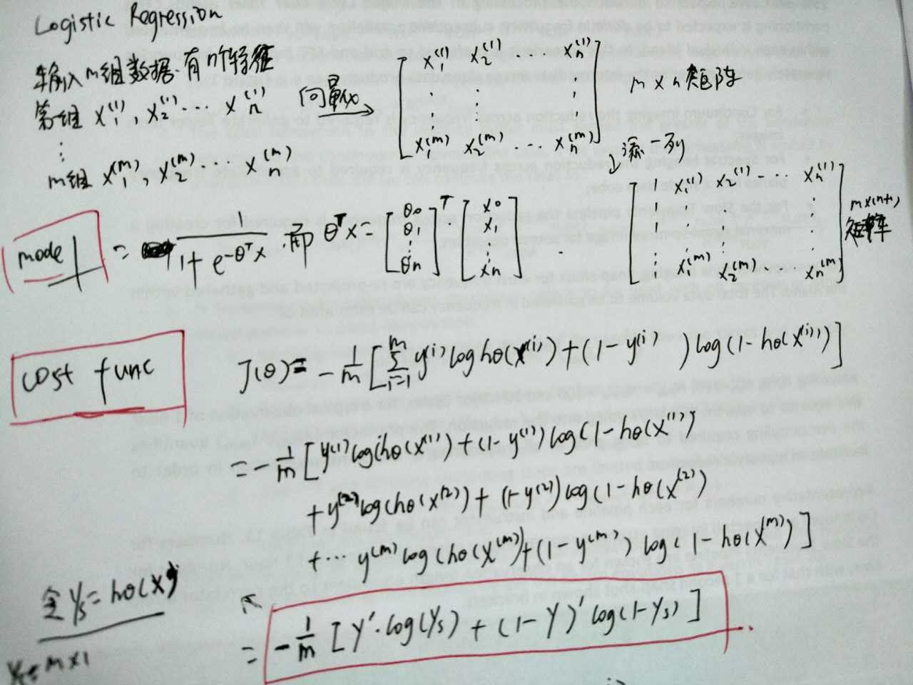
為了使代價函數 $J(\theta)$ 最小化，設假設函數的輸出值 $h_{\theta}(x)$ 與實際值 y 的差為一個趨近于 0 的極小值 $\sigma$ ，則有：

$\sum_{i=1}^{m} (h_\theta(x^{(i)})-y^{(i)})^2=\sigma$ ，

因為 $\sum_{i=1}^{m} (h_\theta(x^{(i)})-y^{(i)})^2=[h(x)-y]^{T}\cdot[(x)-y]$ ，

所以 $(X\theta-y)^{T}(X\theta-y)=\sigma$ ，

兩邊同時對 $\theta$ 求導得： $\theta=\left(X^{T} X\right)^{-1} X^{T} y$

def normalequation(X,y):
    theta=np.linalg.inv(np.dot(X.T,X))@X.T@y
    return theta

final_theta2=normalequation(X, y)#感覺和批量梯度下降的theta的值有點差距
final_theta2

matrix([[-3.89578088],
        [ 1.19303364]])

本文鏈接：https://blog.csdn.net/wyh196646/article/details/101804290

智能推薦

Machine Learning Logistic Regression

機器學習邏輯回歸 1、邏輯回歸與線性回歸的聯系與區別 2、邏輯回歸的原理 3、邏輯回歸損失函數推導及優化 4、正則化與模型評估指標 5、邏輯回歸的優缺點 6、樣本不均衡問題解決辦法 7、sklearn參數 8、代碼實現 1、邏輯回歸與線性回歸的聯系與區別線性回歸解決的是連續變量問題，那么在分類任務中可以用線性回歸嗎？例如判斷是良性腫瘤還是惡性腫瘤，判斷是垃圾郵件還是正常郵件，等等&hellip...

Machine Learning(regression)

Machine Learning 回歸問題一.LinearRegression 二.Ridge(嶺回歸) 三.polyfit(多項式回歸) 四.AdaBoost決策樹與AdaBoost(正向激勵) Feature Importance: 五.randomForestRegressor(隨機森林)...

Machine Learning：Logistic Regression

學習NG的Machine Learning教程，先關推導及代碼。由于在matleb或Octave中需要矩陣或向量，經常搞混淆，因此自己推導，并把向量的形式寫出來了，主要包括cost function及gradient descent 見下圖。圖中可見公式推導，及向量化表達形式的cost function（J）圖中可見公式推導，及向量化表達形式的偏導數。下面為Logistic regressi...

Machine Learning——logistic regression

Machine Learning——logistic regression Problem 1：如何理解coef_和intercept_兩個模型參數 Solution 1：對于線性回歸和邏輯回歸，其目標函數為：f(x) =w0+w1x1+wxx2+… 如果有**函數sigmoid，增加非線性變化，則為分類即邏輯回歸；如果沒有**函數，則為線性回歸。而對于coe...

Machine Learning experiment1 Linear Regression 詳解+源代碼實現

線性回歸回歸模型如下：其中θ是我們需要優化的參數，x是n+1維的特征向量，給定一個訓練集，我們的目標是找出θ的最佳值，使得目標函數J（θ）最小化：優化方法之一是梯度下降算法。算法迭代執行，并在每次迭代中，我們更新θ遵循以下準則其中α是學習率，通過梯度下降的方式，使得損失...

Machine Learning(Andrew Ng）ex1.linear regression

Linear Regression

Linear regression with multiple variables

正規方程法

智能推薦

猜你喜歡