Andrew NG 機器學習 練習2-Logistic Regression
1 Logistic Regression
build a logistic regression model to predict whether a student gets admitted into a university
based on their results on two exams
training set:istorical data from previous applicants
1.1 Visualizing the data
Before starting to implement any learning algorithm, it is always good to visualize the data if possible.
ex2data1.txt(兩科的成績,和是否被錄用)
34.62365962451697,78.0246928153624,0
30.28671076822607,43.89499752400101,0
35.84740876993872,72.90219802708364,0
60.18259938620976,86.30855209546826,1
。。。
%% Load Data
%  The first two columns contains the exam scores and the third column
%  contains the label.

data = load('ex2data1.txt');
X = data(:, [1, 2]); y = data(:, 3);

%% ==================== Part 1: Plotting ====================
%  We start the exercise by first plotting the data to understand the
%  the problem we are working with.

fprintf(['Plotting data with + indicating (y = 1) examples and o ' ...
         'indicating (y = 0) examples.\n']);

plotData(X, y);

% Put some labels
hold on;
% Labels and Legend
xlabel('Exam 1 score')
ylabel('Exam 2 score')

% Specified in plot order
legend('Admitted', 'Not admitted')
hold off;

fprintf('\nProgram paused. Press enter to continue.\n');
pause;
plotData.m
function plotData(X, y)
%PLOTDATA Plots the data points X and y into a new figure
%   PLOTDATA(x,y) plots the data points with + for the positive examples
%   and o for the negative examples. X is assumed to be a Mx2 matrix.

% Create New Figure
figure; hold on;

% ====================== YOUR CODE HERE ======================
% Instructions: Plot the positive and negative examples on a
%               2D plot, using the option 'k+' for the positive
%               examples and 'ko' for the negative examples.
%

%Find Indices of Positive and Negative Examples
pos=find(y==1);%返回y==1的行標 組成的列向量
neg=find(y==0);%返回y==0的行標 組成的列向量

%plot Examples
plot(X(pos,1),X(pos,2),'k+','LineWidth',2,'MarkerSize',7);
plot(X(neg,1),X(neg,2),'ko','MarkerFaceColor','y','MarkerSize',7);
% =========================================================================

hold off;

end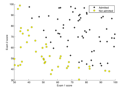
1.2 Implementation
1.2.1 Warmup exercixe:sigmoid function
logistic regression hypothesis is defined as:
g is the sigmoid funciton(S型函數),defined as:
implement this function in sigmoid.m
function g = sigmoid(z)
%SIGMOID Compute sigmoid function
%   g = SIGMOID(z) computes the sigmoid of z.

% You need to return the following variables correctly
g = zeros(size(z));

% ====================== YOUR CODE HERE ======================
% Instructions: Compute the sigmoid of each value of z (z can be a matrix,
%               vector or scalar).

g=1./(1+exp(-z));

% =============================================================

end
1.2.2 Cost function and gradient
the cost function in logistic regression is:
向量方式的實現是:
梯度下降:
模板:
求導后有:
向量方式的實現是:
求的導數值向量:
grad=
costFunction.m
function [J, grad] = costFunction(theta, X, y)
%COSTFUNCTION Compute cost and gradient for logistic regression
%   J = COSTFUNCTION(theta, X, y) computes the cost of using theta as the
%   parameter for logistic regression and the gradient of the cost
%   w.r.t. to the parameters.

% Initialize some useful values
m = length(y); % number of training examples

% You need to return the following variables correctly
J = 0;
grad = zeros(size(theta));

% ====================== YOUR CODE HERE ======================
% Instructions: Compute the cost of a particular choice of theta.
%               You should set J to the cost.
%               Compute the partial derivatives and set grad to the partial
%               derivatives of the cost w.r.t. each parameter in theta
%
% Note: grad should have the same dimensions as theta
%

h=sigmoid(X*theta);
J=1/m*(-y'*log(h)-(1-y)'*log(1-h));

grad = (X' * (sigmoid(X*theta) - y)) ./ m;

% =============================================================

end
%% ============ Part 2: Compute Cost and Gradient ============
%  In this part of the exercise, you will implement the cost and gradient
%  for logistic regression. You neeed to complete the code in
%  costFunction.m

%  Setup the data matrix appropriately, and add ones for the intercept term
[m, n] = size(X);

% Add intercept term to x and X_test
X = [ones(m, 1) X];

% Initialize fitting parameters
initial_theta = zeros(n + 1, 1);

% Compute and display initial cost and gradient
[cost, grad] = costFunction(initial_theta, X, y);

fprintf('Cost at initial theta (zeros): %f\n', cost);
fprintf('Expected cost (approx): 0.693\n');
fprintf('Gradient at initial theta (zeros): \n');
fprintf(' %f \n', grad);
fprintf('Expected gradients (approx):\n -0.1000\n -12.0092\n -11.2628\n');

% Compute and display cost and gradient with non-zero theta
test_theta = [-24; 0.2; 0.2];
[cost, grad] = costFunction(test_theta, X, y);

fprintf('\nCost at test theta: %f\n', cost);
fprintf('Expected cost (approx): 0.218\n');
fprintf('Gradient at test theta: \n');
fprintf(' %f \n', grad);
fprintf('Expected gradients (approx):\n 0.043\n 2.566\n 2.647\n');

fprintf('\nProgram paused. Press enter to continue.\n');
pause;
1.2.3 Learning parameters using fminunc
In the previous assignment, you found the optimal parameters of a linear regression model by implementing gradent descent. You wrote a cost function and calculated its gradient, then took a gradient descent step accordingly.This time, instead of taking gradient descent steps, you will use an Octave/MATLAB built-in function called fminunc.
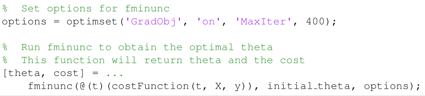
In this code snippet, we first defined the options to be used with fminunc.Specifically, we set the GradObj option to on, which tells fminunc that our function returns both the cost and the gradient. This allows fminunc to use the gradient when minimizing the function. Furthermore, we set the MaxIter option to 400, so that fminunc will run for at most 400 steps before it terminates.
To specify the actual function we are minimizing, we use a “short-hand”for specifying functions with the @(t) ( costFunction(t, X, y) ) . This creates a function, with argument t, which calls your costFunction. This allows us to wrap the costFunction for use with fminunc.
Notice that by using fminunc, you did not have to write any loops yourself, or set a learning rate like you did for gradient descent. This is all done by fminunc: you only needed to provide a function calculating the cost and the gradient.
%% ============= Part 3: Optimizing using fminunc =============
% In this exercise, you will use a built-in function (fminunc) to find the
% optimal parameters theta.
% Set options for fminunc
options = optimset('GradObj', 'on', 'MaxIter', 400);
% Run fminunc to obtain the optimal theta
% This function will return theta and the cost
[theta, cost] = ...
fminunc(@(t)(costFunction(t, X, y)), initial_theta, options);
% Print theta to screen
fprintf('Cost at theta found by fminunc: %f\n', cost);
fprintf('Expected cost (approx): 0.203\n');
fprintf('theta: \n');
fprintf(' %f \n', theta);
fprintf('Expected theta (approx):\n');
fprintf(' -25.161\n 0.206\n 0.201\n');
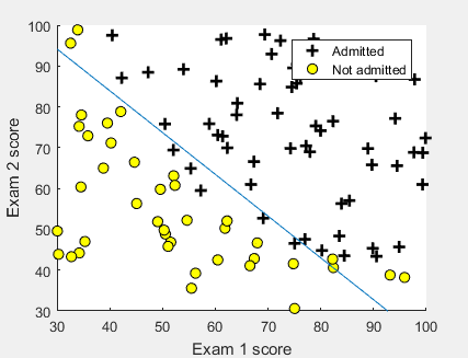
% Plot Boundary
plotDecisionBoundary(theta, X, y);
% Put some labels
hold on;
% Labels and Legend
xlabel('Exam 1 score')
ylabel('Exam 2 score')
% Specified in plot order
legend('Admitted', 'Not admitted')
hold off;
fprintf('\nProgram paused. Press enter to continue.\n');
pause;
plotDecisionBoundary.m
function plotDecisionBoundary(theta, X, y)
%PLOTDECISIONBOUNDARY Plots the data points X and y into a new figure with
%the decision boundary defined by theta
%   PLOTDECISIONBOUNDARY(theta, X,y) plots the data points with + for the
%   positive examples and o for the negative examples. X is assumed to be
%   a either
%   1) Mx3 matrix, where the first column is an all-ones column for the
%      intercept.
%   2) MxN, N>3 matrix, where the first column is all-ones

% Plot Data
plotData(X(:,2:3), y);
hold on

if size(X, 2) <= 3
    % Only need 2 points to define a line, so choose two endpoints
    plot_x = [min(X(:,2))-2,  max(X(:,2))+2];

    % Calculate the decision boundary line
    plot_y = (-1./theta(3)).*(theta(2).*plot_x + theta(1));

    % Plot, and adjust axes for better viewing
    plot(plot_x, plot_y)

    % Legend, specific for the exercise
    legend('Admitted', 'Not admitted', 'Decision Boundary')
    axis([30, 100, 30, 100])
else
    % Here is the grid range
    u = linspace(-1, 1.5, 50);
    v = linspace(-1, 1.5, 50);

    z = zeros(length(u), length(v));
    % Evaluate z = theta*x over the grid
    for i = 1:length(u)
        for j = 1:length(v)
            z(i,j) = mapFeature(u(i), v(j))*theta;
        end
    end
    z = z'; % important to transpose z before calling contour

    % Plot z = 0
    % Notice you need to specify the range [0, 0]
    contour(u, v, z, [0, 0], 'LineWidth', 2)
end
hold off

end
1.2.4 Evaluating logistic regression
%% ============== Part 4: Predict and Accuracies ==============
%  After learning the parameters, you'll like to use it to predict the outcomes
%  on unseen data. In this part, you will use the logistic regression model
%  to predict the probability that a student with score 45 on exam 1 and
%  score 85 on exam 2 will be admitted.
%
%  Furthermore, you will compute the training and test set accuracies of
%  our model.
%
%  Your task is to complete the code in predict.m

%  Predict probability for a student with score 45 on exam 1
%  and score 85 on exam 2

prob = sigmoid([1 45 85] * theta);
fprintf(['For a student with scores 45 and 85, we predict an admission ' ...
         'probability of %f\n'], prob);
fprintf('Expected value: 0.775 +/- 0.002\n\n');

% Compute accuracy on our training set
p = predict(theta, X);

fprintf('Train Accuracy: %f\n', mean(double(p == y)) * 100);%將所有數據放入模型計算,看是否和真實注解一直,來計算模型的準確性
fprintf('Expected accuracy (approx): 89.0\n');
fprintf('\n');
predict.m
function p = predict(theta, X)
%PREDICT Predict whether the label is 0 or 1 using learned logistic
%regression parameters theta
%   p = PREDICT(theta, X) computes the predictions for X using a
%   threshold at 0.5 (i.e., if sigmoid(theta'*x) >= 0.5, predict 1)

m = size(X, 1); % Number of training examples

% You need to return the following variables correctly
p = zeros(m, 1);

% ====================== YOUR CODE HERE ======================
% Instructions: Complete the following code to make predictions using
%               your learned logistic regression parameters.
%               You should set p to a vector of 0's and 1's
%

s=sigmoid(X*theta);
for i=1:m
    if  s(i)>= 0.5
        p(i)=1;
    else
        p(i)=0;
    end
end
%方法二:
% p = floor(sigmoid(X*theta) .* 2)
% =========================================================================

end
2 Regularized logistic regression
預測工廠生產的芯片是否合格
predict whether microchips from a fabrication plant passes quality assurance (QA).
2.1 Visualizing the data
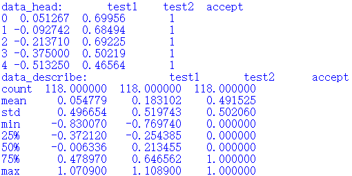
ex2data2.txt
0.051267,0.69956,1
-0.092742,0.68494,1
-0.21371,0.69225,1
-0.375,0.50219,1
-0.51325,0.46564,1
…
數據特征為兩種測試的分數,標簽為 是否可以接受
%% Initialization
clear ; close all; clc

%% Load Data
%  The first two columns contains the X values and the third column
%  contains the label (y).

data = load('ex2data2.txt');
X = data(:, [1, 2]); y = data(:, 3);

plotData(X, y);

% Put some labels
hold on;

% Labels and Legend
xlabel('Microchip Test 1')
ylabel('Microchip Test 2')

% Specified in plot order
legend('y = 1', 'y = 0')
hold off;
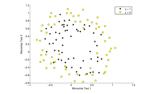
Figure 3 shows that our dataset cannot be separated into positive and negative examples by a straight-line through the plot. Therefore, a straightforward application of logistic regression will not perform well on this dataset since logistic regression will only be able to find a linear decision boundary.
2.2 Feature mapping
One way to fit the data better is to create more features from each data point. In the provided function mapFeature.m, we will map the features into all polynomial terms of x1 and x2 up to the sixth power.
mapFeature(x)=
As a result of this mapping, our vector of two features (the scores on two QA tests) has been transformed into a 28-dimensional vector. A logistic regression classifier trained on this higher-dimension feature vector will have a more complex decision boundary and will appear nonlinear(非線性) when drawn in our 2-dimensional plot.
特征映射可以讓我們構造更富表現力的分類器,但也更易過擬合。
2.3 Cost function and gradient
the regularized cost function in logistic regression is:
Note that you should not regularize the parameter θ0 . (注:根據慣例,我們不對 θ0 進行懲罰。)
要最小化該代價函數,通過求導,得出梯度下降算法為:
注:看上去同線性回歸一樣,但是知道 hθ(x)=g(θTX),所以與線性回歸不同。
%% =========== Part 1: Regularized Logistic Regression ============
%  In this part, you are given a dataset with data points that are not
%  linearly separable. However, you would still like to use logistic
%  regression to classify the data points.
%
%  To do so, you introduce more features to use -- in particular, you add
%  polynomial features to our data matrix (similar to polynomial
%  regression).
%

% Add Polynomial Features

% Note that mapFeature also adds a column of ones for us, so the intercept
% term is handled
X = mapFeature(X(:,1), X(:,2));

% Initialize fitting parameters
initial_theta = zeros(size(X, 2), 1);

% Set regularization parameter lambda to 1
lambda = 1;

% Compute and display initial cost and gradient for regularized logistic
% regression
[cost, grad] = costFunctionReg(initial_theta, X, y, lambda);

fprintf('Cost at initial theta (zeros): %f\n', cost);
fprintf('Expected cost (approx): 0.693\n');
fprintf('Gradient at initial theta (zeros) - first five values only:\n');
fprintf(' %f \n', grad(1:5));
fprintf('Expected gradients (approx) - first five values only:\n');
fprintf(' 0.0085\n 0.0188\n 0.0001\n 0.0503\n 0.0115\n');

fprintf('\nProgram paused. Press enter to continue.\n');
pause;

% Compute and display cost and gradient
% with all-ones theta and lambda = 10
test_theta = ones(size(X,2),1);
[cost, grad] = costFunctionReg(test_theta, X, y, 10);

fprintf('\nCost at test theta (with lambda = 10): %f\n', cost);
fprintf('Expected cost (approx): 3.16\n');
fprintf('Gradient at test theta - first five values only:\n');
fprintf(' %f \n', grad(1:5));
fprintf('Expected gradients (approx) - first five values only:\n');
fprintf(' 0.3460\n 0.1614\n 0.1948\n 0.2269\n 0.0922\n');

fprintf('\nProgram paused. Press enter to continue.\n');
pause;
costFunctionReg.m
function [J, grad] = costFunctionReg(theta, X, y, lambda)
%COSTFUNCTIONREG Compute cost and gradient for logistic regression with regularization
%   J = COSTFUNCTIONREG(theta, X, y, lambda) computes the cost of using
%   theta as the parameter for regularized logistic regression and the
%   gradient of the cost w.r.t. to the parameters.

% Initialize some useful values
m = length(y); % number of training examples

% You need to return the following variables correctly
J = 0;
grad = zeros(size(theta));

% ====================== YOUR CODE HERE ======================
% Instructions: Compute the cost of a particular choice of theta.
%               You should set J to the cost.
%               Compute the partial derivatives and set grad to the partial
%               derivatives of the cost w.r.t. each parameter in theta

h=sigmoid(X*theta);
J=1/m*(-y'*log(h)-(1-y)'*log(1-h))+lambda/(2*m)*(sum(theta.^2) - theta(1)^2);

grad(1)=(X(:,1)' * (h - y)) ./ m;
for i = 2:size(theta)
    grad(i) = (X(:,i)' * (h - y)) ./ m+lambda/m*theta(i);

% =============================================================

end
2.3.1 Learning parameters using fminunc
Similar to the previous parts, you will use fminunc to learn the optimal parameters θ.
%% ============= Part 2: Regularization and Accuracies =============
%  Optional Exercise:
%  In this part, you will get to try different values of lambda and
%  see how regularization affects the decision coundart
%
%  Try the following values of lambda (0, 1, 10, 100).
%
%  How does the decision boundary change when you vary lambda? How does
%  the training set accuracy vary?
%

% Initialize fitting parameters
initial_theta = zeros(size(X, 2), 1);

% Set regularization parameter lambda to 1 (you should vary this)
lambda = 1;

% Set Options
options = optimset('GradObj', 'on', 'MaxIter', 400);

% Optimize
[theta, J, exit_flag] = ...
    fminunc(@(t)(costFunctionReg(t, X, y, lambda)), initial_theta, options);

% Plot Boundary
plotDecisionBoundary(theta, X, y);
hold on;
title(sprintf('lambda = %g', lambda))

% Labels and Legend
xlabel('Microchip Test 1')
ylabel('Microchip Test 2')

legend('y = 1', 'y = 0', 'Decision boundary')
hold off;

% Compute accuracy on our training set
p = predict(theta, X);

fprintf('Train Accuracy: %f\n', mean(double(p == y)) * 100);
fprintf('Expected accuracy (with lambda = 1): 83.1 (approx)\n');
plotDecisionBoundary.m
function plotDecisionBoundary(theta, X, y)
%PLOTDECISIONBOUNDARY Plots the data points X and y into a new figure with
%the decision boundary defined by theta
%   PLOTDECISIONBOUNDARY(theta, X,y) plots the data points with + for the
%   positive examples and o for the negative examples. X is assumed to be
%   a either
%   1) Mx3 matrix, where the first column is an all-ones column for the
%      intercept.
%   2) MxN, N>3 matrix, where the first column is all-ones

% Plot Data
plotData(X(:,2:3), y);
hold on

if size(X, 2) <= 3
    % Only need 2 points to define a line, so choose two endpoints
    plot_x = [min(X(:,2))-2,  max(X(:,2))+2];

    % Calculate the decision boundary line
    plot_y = (-1./theta(3)).*(theta(2).*plot_x + theta(1));

    % Plot, and adjust axes for better viewing
    plot(plot_x, plot_y)

    % Legend, specific for the exercise
    legend('Admitted', 'Not admitted', 'Decision Boundary')
    axis([30, 100, 30, 100])
else
    % Here is the grid range
    u = linspace(-1, 1.5, 50);
    v = linspace(-1, 1.5, 50);

    z = zeros(length(u), length(v));
    % Evaluate z = theta*x over the grid
    for i = 1:length(u)
        for j = 1:length(v)
            z(i,j) = mapFeature(u(i), v(j))*theta;
        end
    end
    z = z'; % important to transpose z before calling contour

    % Plot z = 0
    % Notice you need to specify the range [0, 0]
    contour(u, v, z, [0, 0], 'LineWidth', 2)
end
hold off

end
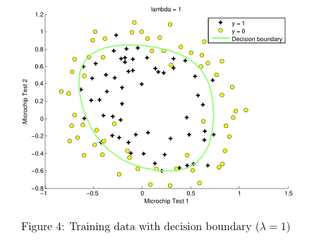
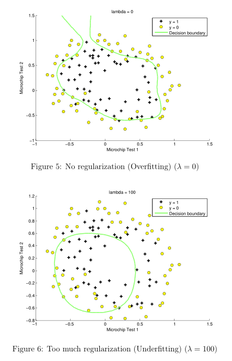
改變 正則化參數 (regularization parameters) λ的值,發現
如果過小,訓練數據擬合的很好,邊界會很復雜,容易過擬合(over fitting),見Figure 5
如果過大,會出現欠擬合(under fitting),見Figure 6
智能推薦
Andrew Ng Machine Learning——Work(Two)——Logistic regression——Regularized(Based on Python 3.7)
所用數據集鏈接:正則化邏輯回歸所用數據(ex2data2.txt),提取碼:c3yy 目錄 Regularized Logistic regression 1.0 Package 1.1 Load data 1.2 Visualization data 1.3 Data preprocess 1.4 Feature mapping 1.5 Sigmoid function 1.6 Regulari...
Andrew Ng 機器學習筆記總結
本文由 CDFMLR 原創,收錄于個人主頁 https://clownote.github.io,并同時發布到 CSDN。本人不保證 CSDN 排版正確,敬請訪問 clownote 以獲得良好的閱讀體驗。 機器學習 Emmmm,這學期在 Coursera 學完了 Andrew Ng 的 Machine Learning 課程。我對這個課程一向是不以為意的,卻不小心報了個名,還手賤申請了個經濟援助,...
Andrew Ng機器學習筆記(五)
一、簡介 二、主要內容 Neural Networks Representation: Non-linear hypothesis: Neurons and the brain: Model representation: Examples and intuitions: Multi-class classification: Cost function: Backpropagation algo...
Andrew Ng機器學習筆記(三)
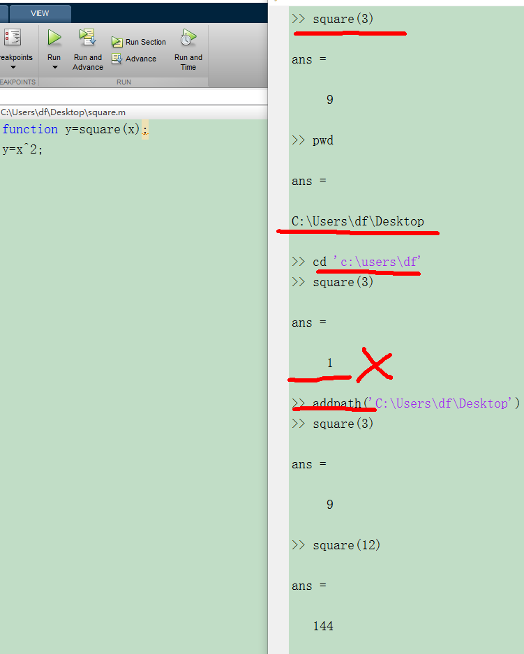
5.matlab教程 原始視頻使用的是Octave語言,與matlab很類似,這里用它代替。 函數路徑問題: 定義一個函數,square,求得是數值的平方。運行結果正確。輸入“pwd”,顯示當前的函數路徑。使用“cd”,修改路徑后,發現函數運行不能顯示正確結果。那么可以考慮,使用’addpath’命令,則函數可以正常運行。當然...

Machine Learning(Andrew Ng)ex1.linear regression
Linear Regression Population Profit 0 6.1101 17.5920 1 5.5277 9.1302 2 8.5186 13.6620 3 7.0032 11.8540 4 5.8598 6.8233 Ones Population 0 1 6.1101 1 1 5.5277 2 1 8.5186 3 1 7.0032 4 1 5.8598 Profit 0 1...
猜你喜歡
Andrew NG 機器學習 練習8-Anomaly Detection and Recommender Systems
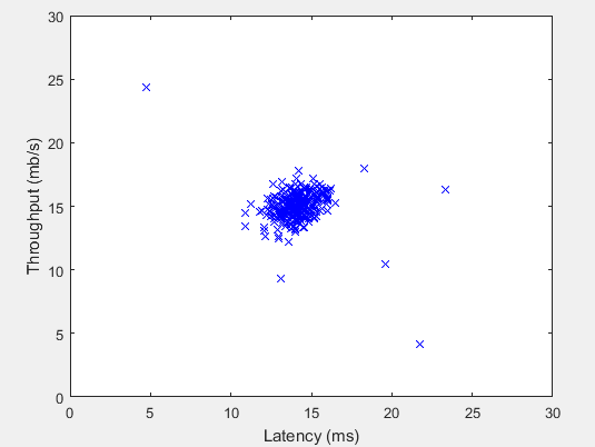
1 Anomaly detection 實現一個異常檢測算法檢測服務器的異常行為 特征是 每個服務器的 吞吐量(throughput)(mb/s) 和 相應延遲(ms) 采集 m=307 臺運行中的服務器的特征,{x(1),...,x(m)} 其中大部分是 normal 的服務器特征 你將使用 高斯模型 檢測數據集中的異常樣例 從 2D 數據集開始,以便可視化算法過程 在那個數據集中你將擬合一個高...
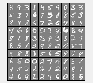
Andrew NG 機器學習 練習3-Multiclass Classification and Neural Networks
In this exercise, you will implement one-vs-all logistic regression and neural networks to recognize hand-written digits. 1 Multi-class Classification In the first part of the exercise, you will exten...
ML - Coursera Andrew Ng - Week1 & Week2 & Ex1 - Linear Regression - 筆記與代碼
Week 1和Week 2主要講解了機器學習中的一些基礎概念,并介紹了線性回歸算法(Linear Regression)。 機器學習主要分為三類: 監督學習(Supervised Learning):已知給定輸入的數據集的輸出結果。監督學習是學習輸入和輸出之間的映射關系。根據輸出值的類型監督學習問題可分為回歸(regression)問題和分類(classification)問題。如果輸出值是連續的...


freemarker + ItextRender 根據模板生成PDF文件
1. 制作模板 2. 獲取模板,并將所獲取的數據加載生成html文件 2. 生成PDF文件 其中由兩個地方需要注意,都是關于獲取文件路徑的問題,由于項目部署的時候是打包成jar包形式,所以在開發過程中時直接安照傳統的獲取方法沒有一點文件,但是當打包后部署,總是出錯。于是參考網上文章,先將文件讀出來到項目的臨時目錄下,然后再按正常方式加載該臨時文件; 還有一個問題至今沒有解決,就是關于生成PDF文件...