代碼標注及運行、調試結果
tips:深度學習中的很多錯誤軟件來自矩陣/向量的維度不匹配,要注意檢查
1.準備工作
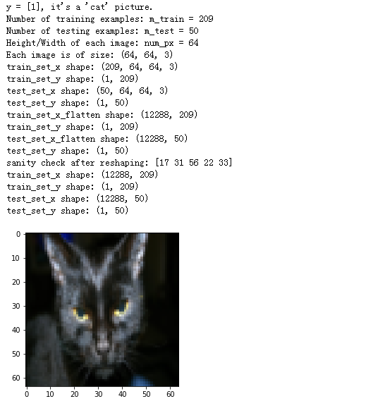
import numpy as np '''python用于科學計算的基礎包'''

import matplotlib.pyplot as plt '''python中繪制圖形的庫'''

import h5py '''與存儲在H5文件中的數據集交互的常見包'''

import scipy
from PIL import Image
from scipy import ndimage
from lr_utils import load_dataset

%matplotlib inline

###加載設置好的數據集###

train_set_x_orig, train_set_y, test_set_x_orig, test_set_y, classes = load_dataset()
index = 25

plt.imshow(train_set_x_orig[index])
print ("y = " + str(train_set_y[:, index]) + ", it's a '" + classes[np.squeeze(train_set_y[:, index])].decode("utf-8") + "' picture.")


###train_set_x_orig的數組形式:shape (m_train, num_px, num_px, 3)

#例如可以通過訪問:train_set_x_orig.shape[0] 訪問到m_train(訓練數量)
###應用###
m_train = train_set_x_orig.shape[0]
m_test = test_set_x_orig.shape[0]
num_px = train_set_x_orig.shape[1]


print ("Number of training examples: m_train = " + str(m_train))
print ("Number of testing examples: m_test = " + str(m_test))
print ("Height/Width of each image: num_px = " + str(num_px))
print ("Each image is of size: (" + str(num_px) + ", " + str(num_px) + ", 3)")
print ("train_set_x shape: " + str(train_set_x_orig.shape))
print ("train_set_y shape: " + str(train_set_y.shape))
print ("test_set_x shape: " + str(test_set_x_orig.shape))
print ("test_set_y shape: " + str(test_set_y.shape))

#轉化訓練和測試用例
###想要將一個形如(a,b,c,d)的矩陣轉化為 (b ?? c ?? d, a) 的矩陣,使用X_flatten = X.reshape(X.shape[0], -1).T 其中X.T 是X的矩陣的轉置###


###應用###
train_set_x_flatten = train_set_x_orig.reshape(train_set_x_orig.shape[0], -1).T
test_set_x_flatten = test_set_x_orig.reshape(test_set_x_orig.shape[0], -1).T


print ("train_set_x_flatten shape: " + str(train_set_x_flatten.shape))
print ("train_set_y shape: " + str(train_set_y.shape))
print ("test_set_x_flatten shape: " + str(test_set_x_flatten.shape))
print ("test_set_y shape: " + str(test_set_y.shape))
print ("sanity check after reshaping: " + str(train_set_x_flatten[0:5,0])) #???????

#要表示彩色圖像,必須為每個像素指定紅色,綠色和藍色通道(RGB),因此像素值實際上是包含三個數字的向量,范圍從0到255。
#機器學習中一個常見的預處理步驟是對數據集進行居中和標準化,這意味著您從每個示例中減去整個numpy數組的平均值,
#然后將每個示例除以整個numpy數組的標準偏差。 但是對于圖片數據集,它更簡單,更方便,幾乎可以將數據集的每一行除以255(像素通道的最大值)。
#將我們的數據集進行標準化。

train_set_x = train_set_x_flatten/255.
test_set_x = test_set_x_flatten/255.

print ("train_set_x shape: " + str(train_set_x.shape))
print ("train_set_y shape: " + str(train_set_y.shape))
print ("test_set_x shape: " + str(test_set_x.shape))
print ("test_set_y shape: " + str(test_set_y.shape))
###預處理新數據集的常用步驟如下:
###弄清楚問題的大小和形狀(m_train,m_test,num_px,...)
###重塑數據集,使每個示例是一個大小為(num_px * num_px * 3,1)的向量的“標準化”數據
結果:
2.數組訪問技巧
train_set_x_orig的數組形式:shape (m_train, num_px, num_px, 3)

#例如可以通過訪問:train_set_x_orig.shape[0] 訪問到m_train(訓練數量)
3.學習算法的一般體系結構
設計一種簡單的算法來區分貓圖像和非貓圖像。
您將使用神經網絡思維模式構建Logistic回歸。 下圖解釋了為什么Logistic回歸實際上是一個非常簡單的神經網絡!

數學表達式:
針對樣例
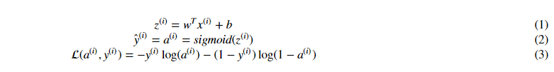
cost函數:

接下來完成以下步驟:
- 初始化模型的參數
- 通過最小化成本來了解模型的參數
- 使用學習的參數進行預測(在測試集上)
- 分析結果并得出結論
4.開始構建算法的各個部分
構建神經網絡的主要步驟是:
定義模型結構(例如輸入元素的數量)
初始化模型的參數
循環:
計算當前loss函數(前向傳播)
計算當前梯度(反向傳播)
更新參數(梯度下降)
經常會單獨構建以上三個循環,并將它們集成到一個我們稱為model()的函數中。
4.1 幫助函數
使用“Python Basics”中的代碼,實現sigmoid(),通過計算sigmoid,對其  進行預測,其中建議使用np.exp()
import numpy as np

def sigmoid(z):
    """
    計算z的sigmoid函數

    參數:
    z -- 任意大小的數組或者常量.

    返回值:
    s -- sigmoid(z)
    """

    ###應用###
    s = 1 / (1 + np.exp(-z))
    ###s = (1 + np.exp(-z))**(-1)  也可以

    return s
    #函數輸出的測試(可以通過數組的方式一次輸入多個)
print ("sigmoid([3, 0]) = " + str(sigmoid(np.array([3,0]))))
4.2 初始化參數
如果輸入的是圖片,則w的維度設置為 (num_px ×× num_px ×× 3, 1).
將w初始化為0,建議使用np.zeros() ,b的值根據實際情況進行設置
import numpy as np
def initialize_with_zeros(dim):
    """
    該函數創建一個維數為(dim,1),元素值為0的列向量,將b初始化為0
    參數:
    dim -- 我們想要設置的w向量的大小(或者是用例中的參數個數)

    返回值:
    w -- 初始化為 (dim, 1)的向量
    b -- 初始化標量(對應于偏差)
    """

    ### 應用###
    w = np.zeros((dim, 1), dtype=np.float)  #dtype指定數據類型
    b = 9
    #檢測
    assert(w.shape == (dim, 1))
    assert(isinstance(b, float) or isinstance(b, int))

    return w, b
驗證輸出:
dim = 7
w, b = initialize_with_zeros(dim)
print ("w = " + str(w))
print ("b = " + str(b))
4.3前向和反向傳播
目前參數已經進行初始化了,接下來可以通過執行前向和反向傳播步驟進一步學習參數
實現propagate() 函數,計算cost函數以及他的梯度下降
提示:
前向傳播:
1) 獲得X矩陣
2)計算
3)計算cost函數 
可能用到的公式:
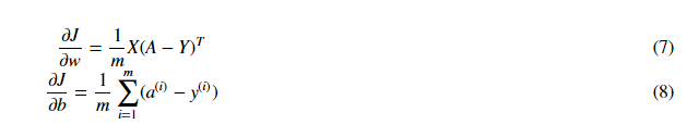
# 前向傳播函數
import numpy as np

def sigmoid(z):


    ###應用###
    s = 1 / (1 + np.exp(-z))
    ###s = (1 + np.exp(-z))**(-1)  也可以

    return s
def propagate(w, b, X, Y):
    """
    參數:
    w -- 權重,大小為(num_px * num_px * 3, 1)的數組
    b -- 偏差, 是個常量
    X -- 數據大小 (num_px * num_px * 3, 樣本大小)
    Y --  "label" 向量(0表示不是貓, 1表示是貓),其維數為(1, 樣本大小)

    返回值:
    cost -- 公式計算得出的值
    dw -- loss對w的導數, 因此維數與w一樣
    db -- loss對b的導數, 因此維數與b一樣

    提示:
    - 建議使用 np.log(), np.dot()
    """

    m = X.shape[1]

    #前向
    ### 應用np里面的內置函數
    A = sigmoid(np.dot(w.T,X)+b)                                  #計算**函數
    cost =-1/m * np.sum(Y * np.log(A)+(1-Y)*np.log(1-A))                                  #計算cost函數,注意負號和A
    # 反向
    ###注意.dot的使用
    dw = 1/m*(np.dot(X,(A-Y).T))
    db = 1/m*np.sum(A-Y)
    ### END CODE HERE ###

    assert(dw.shape == w.shape)
    assert(db.dtype == float)
    cost = np.squeeze(cost)
    assert(cost.shape == ())

    grads = {"dw": dw,
             "db": db}

    return grads, cost
驗證輸出:
w, b, X, Y = np.array([[1.],[2.]]), 2., np.array([[1.,2.,-1.],[3.,4.,-3.2]]), np.array([[1,0,1]])
grads, cost = propagate(w, b, X, Y)
print ("dw = " + str(grads["dw"]))
print ("db = " + str(grads["db"]))
print ("cost = " + str(cost))
4.4優化函數
目前已經初始化參數、計算cost函數及其梯度,現在要做的是使用梯度下降更新參數。
構造優化函數,通過最小化cost函數J,找到合適的w和b的值
對于參數θ,更新規則是θ=θ-αdθ,其中α為學習率
def optimize(w, b, X, Y, num_iterations, learning_rate, print_cost = False):
    """
    通過梯度下降算法,優化參數w和b
    參數:
    w -- 權重,大小為(num_px * num_px * 3, 1)的數組
    b -- 偏差, 是個常量
    X -- 數據大小 (num_px * num_px * 3, 樣本大小)
    Y --  "label" 向量(0表示不是貓, 1表示是貓),其維數為(1, 樣本大小)
    num_iterations -- 優化循環的迭代次數
    learning_rate --梯度下降更新規則的學習率
    print_cost --每100步打印一次loss函數

    返回值:
    params -- 一個dictionary 包含權重w和偏差b
    grads --  一個dictionary 包含所期望的cost函數中的權重的導數dw和偏差的導數db
    costs --  一個list       包含優化過程中計算的所有的cost函數值,用于繪制學習曲線

    提示:
    主要包含以下兩個步驟并進行迭代:
       1)使用propagate() 計算當前參數的cost函數和梯度
       2)使用梯度下降規則中的w和b更新參數
    """

    costs = []

    for i in range(num_iterations):


        ###調用前向傳播函數###
        grads, cost = propagate(w, b, X, Y)


        # Retrieve derivatives from grads
        dw = grads["dw"]
        db = grads["db"]
        #更新規則
        ###注意轉化為矩陣的相乘的形式###
        w = w - np.dot(learning_rate, dw)
        b = b - np.dot(learning_rate, db)


        # Record the costs
        if i % 100 == 0:
            costs.append(cost)

        # Print the cost every 100 training examples
        if print_cost and i % 100 == 0:
            print ("Cost after iteration %i: %f" %(i, cost))

    params = {"w": w,
              "b": b}

    grads = {"dw": dw,
             "db": db}

    return params, grads, costs
仍然使用前面設定的值對函數進行結果測試:
params, grads, costs = optimize(np.array([[1.],[2.]]), 2., np.array([[1.,2.,-1.],[3.,4.,-3.2]]), np.array([[1,0,1]]), num_iterations= 100, learning_rate = 0.009, print_cost = False)

print ("w = " + str(params["w"]))
print ("b = " + str(params["b"]))
print ("dw = " + str(grads["dw"]))
print ("db = " + str(grads["db"]))
前面的函數將輸出最終學習的w和b,我們可以用w和b的值去預測數據集X的標簽,應用predict()函數,主要分為兩個步驟來計算預測值
1.計算 
2.將a的值轉換成0(**函數<=0.5)或1(**函數>0.5),將預測值存儲在向量Y_prediction中(也可以通過在for循環中使用if...else實現)
# GRADED FUNCTION: predict

def predict(w, b, X):
    '''
    使用學習到的logistic 回歸參數(w,b)來預測標簽值是0還是1
    參數:
    w -- 權重,大小為(num_px * num_px * 3, 1)的數組
    b -- 偏差, 是個常量
    X -- 數據大小 (num_px * num_px * 3, 樣本大小)

    返回值:
    Y_prediction -- 包含在X中的樣本的所有預測值,是一個數組或者向量
    '''

    m = X.shape[1]
    Y_prediction = np.zeros((1,m))
    w = w.reshape(X.shape[0], 1)

    # Compute vector "A" predicting the probabilities of a cat being present in the picture
    ### START CODE HERE ###
    A = sigmoid(np.dot(w.T, X) + b)
    ### END CODE HERE ###
    print(A.shape[1])
    for i in range(A.shape[1]):
        if A[0,i] <= 0.5:
            Y_prediction[0, i] = 0
        else:
            Y_prediction[0, i] = 1
        # Convert probabilities A[0,i] to actual predictions p[0,i]
        ### START CODE HERE ### (≈ 4 lines of code)
        ### END CODE HERE ###

    assert(Y_prediction.shape == (1, m))

    return Y_prediction
驗證輸出:
w = np.array([[0.1124579],[0.23106775]])
b = -0.3
X = np.array([[1.,-1.1,-3.2],[1.2,2.,0.1]])
print ("predictions = " + str(predict(w, b, X)))
5.將所有函數合并到模型中
通過以下提示,實現模型函數:
--Y_prediction_test 測試集上的預測值
--Y_prediction_train 訓練集上的預測值
--optimize() 優化輸出的 w,costs,grads 值
# GRADED FUNCTION: model
def sigmoid(z):

    ###應用###
    s = 1 / (1 + np.exp(-z))
    ###s = (1 + np.exp(-z))**(-1)  也可以

    return s
def initialize_with_zeros(dim):

    w = np.zeros((dim,1))
    b = 9

    assert(w.shape == (dim, 1))
    assert(isinstance(b, float) or isinstance(b, int))

    return w, b
def propagate(w, b, X, Y):

    m = X.shape[1]

    #前向
    ### 應用np里面的內置函數
    A = sigmoid(np.dot(w.T,X)+b)                                  #計算**函數
    cost =-1/m * np.sum(Y * np.log(A)+(1-Y)*np.log(1-A))                                  #計算cost函數,注意負號和A
    # 反向
    ###注意.dot的使用
    dw = 1/m*(np.dot(X,(A-Y).T))
    db = 1/m*np.sum(A-Y)
    ### END CODE HERE ###

    assert(dw.shape == w.shape)
    assert(db.dtype == float)
    cost = np.squeeze(cost)
    assert(cost.shape == ())

    grads = {"dw": dw,
             "db": db}

    return grads, cost
def optimize(w, b, X, Y, num_iterations, learning_rate, print_cost = False):

    costs = []

    for i in range(num_iterations):

        ###調用前向傳播函數###
        grads, cost = propagate(w, b, X, Y)


        # Retrieve derivatives from grads
        dw = grads["dw"]
        db = grads["db"]
        #更新規則
        ###注意轉化為矩陣的相乘的形式###
        w = w - np.dot(learning_rate, dw)
        b = b - np.dot(learning_rate, db)


        # Record the costs
        if i % 100 == 0:
            costs.append(cost)

        # Print the cost every 100 training examples
        if print_cost and i % 100 == 0:
            print ("Cost after iteration %i: %f" %(i, cost))

    params = {"w": w,
              "b": b}

    grads = {"dw": dw,
             "db": db}

    return params, grads, costs
def predict(w, b, X):

    m = X.shape[1]
    Y_prediction = np.zeros((1,m))
    w = w.reshape(X.shape[0], 1)

    # Compute vector "A" predicting the probabilities of a cat being present in the picture
    ### START CODE HERE ###
    A = sigmoid(np.dot(w.T, X) + b)
    ### END CODE HERE ###
    print(A.shape[1])
    for i in range(A.shape[1]):
        if A[0,i] <= 0.5:
            Y_prediction[0, i] = 0
        else:
            Y_prediction[0, i] = 1
        # Convert probabilities A[0,i] to actual predictions p[0,i]
        ### START CODE HERE ### (≈ 4 lines of code)
        ### END CODE HERE ###

    assert(Y_prediction.shape == (1, m))

    return Y_prediction

def model(X_train, Y_train, X_test, Y_test, num_iterations = 2000, learning_rate = 0.5, print_cost = False):
    """
    通過調用之前實現的函數構建logistic回歸模型

    參數:
    X_train -- 維數為 (num_px * num_px * 3, m_train) 的訓練集
    Y_train -- 維數為 (1, m_train) 的訓練標簽
    X_test --  維數為 (num_px * num_px * 3, m_test) 的測試集
    Y_test --  維數為(1, m_test) 的測試標簽
    num_iterations -- 超參數,表示優化參數的迭代次數
    learning_rate --  超參數,表示在optimize()更新規則中使用的學習率
    print_cost --  設置為true,以每100次迭代打印cost函數的值

    返回值:
    d -- 一個dictionary,包含一個模型的基本信息.
    """

    ### START CODE HERE ###

    # initialize parameters with zeros (≈ 1 line of code)
    w, b = initialize_with_zeros(X_train.shape[0])

    # Gradient descent (≈ 1 line of code)
    parameters, grads, costs = optimize(w, b, X_train, Y_train, num_iterations, learning_rate, print_cost)

    # Retrieve parameters w and b from dictionary "parameters"
    w = parameters["w"]
    b = parameters["b"]

    # Predict test/train set examples (≈ 2 lines of code)
    Y_prediction_test = predict(w, b, X_test)
    Y_prediction_train = predict(w, b, X_train)

    ### END CODE HERE ###

    # Print train/test Errors
    print("train accuracy: {} %".format(100 - np.mean(np.abs(Y_prediction_train - Y_train)) * 100))
    print("test accuracy: {} %".format(100 - np.mean(np.abs(Y_prediction_test - Y_test)) * 100))


    d = {"costs": costs,
         "Y_prediction_test": Y_prediction_test,
         "Y_prediction_train" : Y_prediction_train,
         "w" : w,
         "b" : b,
         "learning_rate" : learning_rate,
         "num_iterations": num_iterations}

    return d
驗證輸出:
import numpy as np
import matplotlib.pyplot as plt
import h5py
import scipy
from PIL import Image
from scipy import ndimage
from lr_utils import load_dataset

%matplotlib inline

train_set_x_orig, train_set_y, test_set_x_orig, test_set_y, classes = load_dataset()
index = 25
###plt.imshow(test_set_x_orig[index])###
plt.imshow(train_set_x_orig[index])
print ("y = " + str(train_set_y[:, index]) + ", it's a '" + classes[np.squeeze(train_set_y[:, index])].decode("utf-8") +  "' picture.")


###train_set_x_orig的數組形式:shape (m_train, num_px, num_px, 3)

#例如可以通過訪問:train_set_x_orig.shape[0]  訪問到m_train(訓練數量)
### START CODE HERE ### (≈ 3 lines of code)
m_train = train_set_x_orig.shape[0]
m_test = test_set_x_orig.shape[0]
num_px = train_set_x_orig.shape[1]
### END CODE HERE ###

### START CODE HERE ### (≈ 2 lines of code)
train_set_x_flatten = train_set_x_orig.reshape(train_set_x_orig.shape[0], -1).T
test_set_x_flatten = test_set_x_orig.reshape(test_set_x_orig.shape[0], -1).T
### END CODE HERE ###

train_set_x = train_set_x_flatten/255.
test_set_x = test_set_x_flatten/255.

print ("train_set_x shape: " + str(train_set_x.shape))
print ("train_set_y shape: " + str(train_set_y.shape))
print ("test_set_x shape: " + str(test_set_x.shape))
print ("test_set_y shape: " + str(test_set_y.shape))

d = model(train_set_x, train_set_y, test_set_x, test_set_y, num_iterations = 2000, learning_rate = 0.005, print_cost = True)
輸出:
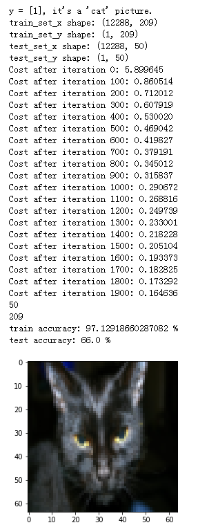
分析:訓練正確率接近100%。有一個不錯的完整性檢查:您的模型正在運行,并且具有足夠的容量來適應訓練數據。測試錯誤率約為40%(?),對于這個簡單模型是可以接受的,我們使用的是比較少的數據集而且logistic回歸是一個線性分類器,下周將嘗試更加準確的分類器
此外,可以看出,模型顯然過度擬合了訓練數據,之后將學習如何減少過擬合,例如:使用正規化,使用以下代碼并改變index的值,可以看到測試集的預測值
增加迭代次數,進行測試:
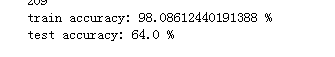
d = model(train_set_x, train_set_y, test_set_x, test_set_y, num_iterations = 3000, learning_rate = 0.005, print_cost = True) #更改 num_iterations = 3000 參數
部分結果:
繪制學習率曲線:

解釋:可以看出cost函數不斷下降,這表明各項參數正在被學習。你會發現你可以在訓練集上訓練模型,試著增加上述單元的迭代次數并返回,會發現訓練集的正確率增加,但是測試集的正確率下降,稱之為過擬合(overfitting)
6.附加題1
通過以下提示,實現模型函數,測試學習率α可能的值
提示:為了使得梯度下降更有效,應選擇更加合適的學習率,學習率α決定了是否能快速更新參數。學習率過大,可能會“超”過最佳值,學習率過小,將需要更多的迭代來收斂(收斂)到最佳值。這就是為何選擇一個“精調”的學習率的至關重要的原因
運行以下代碼,輸入不同的學習率,觀察結果:
learning_rates = [0.01, 0.001, 0.0001]
models = {}
for i in learning_rates:
    print ("learning rate is: " + str(i))
    models[str(i)] = model(train_set_x, train_set_y, test_set_x, test_set_y, num_iterations = 1500, learning_rate = i, print_cost = False)
    print ('\n' + "-------------------------------------------------------" + '\n')

for i in learning_rates:
    plt.plot(np.squeeze(models[str(i)]["costs"]), label= str(models[str(i)]["learning_rate"]))

plt.ylabel('cost')
plt.xlabel('iterations (hundreds)')

legend = plt.legend(loc='upper center', shadow=True)
frame = legend.get_frame()
frame.set_facecolor('0.90')
plt.show()

解釋:
1)不同的學習率會得到不同的cost值,因此會有不同的預測結果
2)如果學習率過大(0.01),cost值將上下擺動,甚至會偏離(即使在這個例子中,使用0.01能最終收斂到cost的一個合適的值)
3)cost值小不代表是一個好模型,必須檢查會不會有可能過擬合,過擬合經常發生在訓練正確率比測試正確率大很多的情況下
4)在深度學習中,強烈推薦:
選擇合適的學習率來使cost函數盡可能小
如果你的模型過擬合,選擇其他技術來減少過擬合(之后繼續學習)
7.附加題2
自己添加圖片,測試模型如何處理:
總結:
1)對數據集進行預處理很重要
2)分別實現每個函數功能,再將其合并到一個model()函數中
3)調整學習率(這是“超參數”的一個例子)可以給算法帶來很大不同,后面將看到更多的例子。