Machine Learning(Andrew Ng)ex2.logistic regression
import pandas as pd
import numpy as np
import matplotlib.pyplot as plt
import seaborn as sns
from sklearn.metrics import classification_report
data=pd.read_csv('ex2data1.txt',header=None,names=['Exam1','Exam2','Admitted'])
data.head()
| Exam1 | Exam2 | Admitted | |
|---|---|---|---|
| 0 | 34.623660 | 78.024693 | 0 |
| 1 | 30.286711 | 43.894998 | 0 |
| 2 | 35.847409 | 72.902198 | 0 |
| 3 | 60.182599 | 86.308552 | 1 |
| 4 | 79.032736 | 75.344376 | 1 |
data.head()
| Exam1 | Exam2 | Admitted | |
|---|---|---|---|
| 0 | 34.623660 | 78.024693 | 0 |
| 1 | 30.286711 | 43.894998 | 0 |
| 2 | 35.847409 | 72.902198 | 0 |
| 3 | 60.182599 | 86.308552 | 1 |
| 4 | 79.032736 | 75.344376 | 1 |
positive=data[data['Admitted'].isin([1])]#用法有待考究
negative=data[data['Admitted'].isin([0])]
positive.head()
data['Admitted'].isin([1]).head()
0    False
1    False
2    False
3     True
4     True
Name: Admitted, dtype: bool
positive.head()
| Exam1 | Exam2 | Admitted | |
|---|---|---|---|
| 3 | 60.182599 | 86.308552 | 1 |
| 4 | 79.032736 | 75.344376 | 1 |
| 6 | 61.106665 | 96.511426 | 1 |
| 7 | 75.024746 | 46.554014 | 1 |
| 8 | 76.098787 | 87.420570 | 1 |
sns.set(context='notebook',style='darkgrid')
sns.lmplot('Exam1','Exam2',hue='Admitted',data=data,fit_reg=False)
<seaborn.axisgrid.FacetGrid at 0x1d1d7c26e10>

def sigmoid(z):
    return 1/(1+np.exp(-z))
def get_X(df):
    data.insert(0,'Ones',1)
    return data.iloc[:, :-1].as_matrix()

def get_y(df):
    return np.array(df.iloc[:,-1])

def normalize_feature(df):
    df=(df-df.mean())/df.std()
    return df
theta=np.zeros(3)
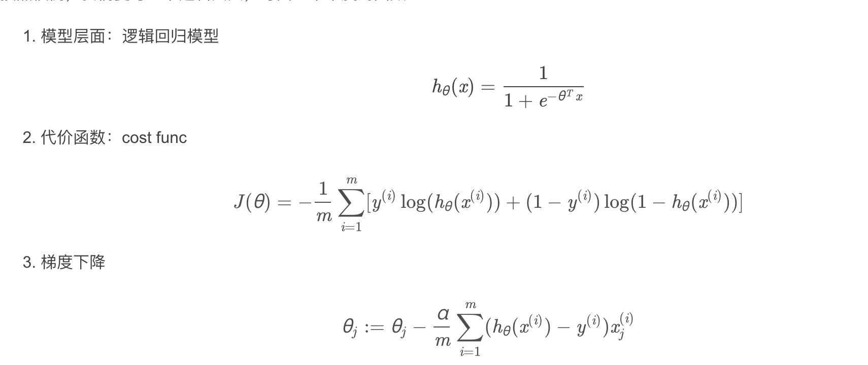
Logisc Regression cost function
def cost(theta,X,y):#@代表矩陣乘法
    return np.mean(-y*np.log(sigmoid(X@theta))-(1-y)*np.log(1-sigmoid(X@theta)))
X=get_X(data)
y=get_y(data)
c:\users\19664\appdata\local\programs\python\python37\lib\site-packages\ipykernel_launcher.py:3: FutureWarning: Method .as_matrix will be removed in a future version. Use .values instead.
  This is separate from the ipykernel package so we can avoid doing imports until
cost(theta,X,y)
0.6931471805599453
gradient descent(梯度下降)
- 這是批量梯度下降(batch gradient descent)
- 轉化為向量化計算:
def gradient_decent(theta, x, y):
#     '''just 1 batch gradient'''
    return (1 / len(x)) * (((sigmoid(x @ theta) - y).T) @ x)
gradient_decent(theta,X,y)
array([ -0.1 , -12.00921659, -11.26284221])
import scipy
import scipy.optimize as opt
res=opt.minimize(fun=cost,x0=theta,args=(X,y),method='Newton-CG', jac=gradient_decent)
print(res)
     fun: 0.20349770628264552
     jac: array([-5.89271913e-06, -4.23590443e-04, -5.16057328e-04])
 message: 'Optimization terminated successfully.'
    nfev: 71
    nhev: 0
     nit: 28
    njev: 242
  status: 0
 success: True
       x: array([-25.15571627,   0.20618678,   0.20142615])
訓練集預測檢驗
def predict(x,theta):
        h=sigmoid(x@theta)
        return (h >= 0.5).astype(int)#用法有待考究
尋找決策邊界
\[{{h}_{\theta }}\left( x \right)=\frac{1}{1+{{e}^{-{{\theta }^{T}}X}}}\]
coef = -(res.x / res.x[2])
x = np.arange(130, step=0.1)
y = coef[0] + coef[1]*x
sns.set(context='notebook',style='darkgrid')
sns.lmplot('Exam1','Exam2',hue='Admitted',data=data,fit_reg=False)
plt.plot(x, y, 'r')
plt.xlim(0, 130)
plt.ylim(0, 130)
plt.title('Decision Boundary')
plt.show()

邏輯化正則回歸(處理關系過擬合的問題)
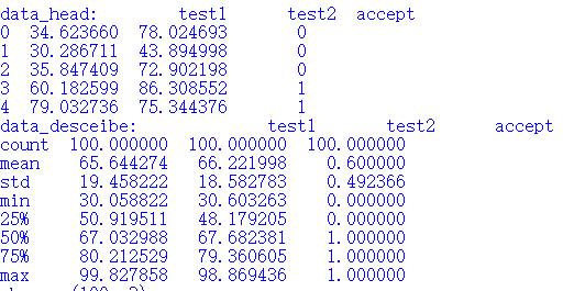
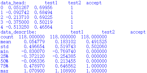
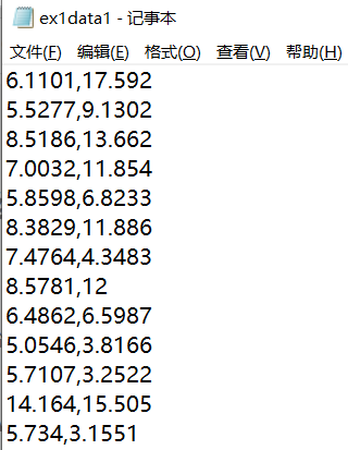
data2=pd.read_csv('ex2data2.txt',names=['test1','test2','accepted'])
data2.head()
| test1 | test2 | accepted | |
|---|---|---|---|
| 0 | 0.051267 | 0.69956 | 1 |
| 1 | -0.092742 | 0.68494 | 1 |
| 2 | -0.213710 | 0.69225 | 1 |
| 3 | -0.375000 | 0.50219 | 1 |
| 4 | -0.513250 | 0.46564 | 1 |
sns.set(context='notebook',style='darkgrid')
sns.lmplot('test1','test2',hue='accepted',data=data2,fit_reg=False)
<seaborn.axisgrid.FacetGrid at 0x1d1dad38588>

data2.head()
| test1 | test2 | accepted | |
|---|---|---|---|
| 0 | 0.051267 | 0.69956 | 1 |
| 1 | -0.092742 | 0.68494 | 1 |
| 2 | -0.213710 | 0.69225 | 1 |
| 3 | -0.375000 | 0.50219 | 1 |
| 4 | -0.513250 | 0.46564 | 1 |
feature mapping(特征擴張,構造多項式特征)
def feature_mapping(x1,x2,power):#特征映射,創造新特征
    data=pd.DataFrame()
    for i in range(power+1):#for i in range(0)這個是1坑,遵從左開右閉的規則
        for j in range(0,i+1):
            data['F' + str(j) + str(i)] = np.power(x1, i-j) * np.power(x2, j)
    return data
x1=np.array(data2.test1)
x2=np.array(data2.test2)
data_3=feature_mapping(x1,x2,6)
data_3.head()
| F00 | F01 | F11 | F02 | F12 | F22 | F03 | F13 | F23 | F33 | ... | F35 | F45 | F55 | F06 | F16 | F26 | F36 | F46 | F56 | F66 | |
|---|---|---|---|---|---|---|---|---|---|---|---|---|---|---|---|---|---|---|---|---|---|
| 0 | 1.0 | 0.051267 | 0.69956 | 0.002628 | 0.035864 | 0.489384 | 0.000135 | 0.001839 | 0.025089 | 0.342354 | ... | 0.000900 | 0.012278 | 0.167542 | 1.815630e-08 | 2.477505e-07 | 0.000003 | 0.000046 | 0.000629 | 0.008589 | 0.117206 |
| 1 | 1.0 | -0.092742 | 0.68494 | 0.008601 | -0.063523 | 0.469143 | -0.000798 | 0.005891 | -0.043509 | 0.321335 | ... | 0.002764 | -0.020412 | 0.150752 | 6.362953e-07 | -4.699318e-06 | 0.000035 | -0.000256 | 0.001893 | -0.013981 | 0.103256 |
| 2 | 1.0 | -0.213710 | 0.69225 | 0.045672 | -0.147941 | 0.479210 | -0.009761 | 0.031616 | -0.102412 | 0.331733 | ... | 0.015151 | -0.049077 | 0.158970 | 9.526844e-05 | -3.085938e-04 | 0.001000 | -0.003238 | 0.010488 | -0.033973 | 0.110047 |
| 3 | 1.0 | -0.375000 | 0.50219 | 0.140625 | -0.188321 | 0.252195 | -0.052734 | 0.070620 | -0.094573 | 0.126650 | ... | 0.017810 | -0.023851 | 0.031940 | 2.780914e-03 | -3.724126e-03 | 0.004987 | -0.006679 | 0.008944 | -0.011978 | 0.016040 |
| 4 | 1.0 | -0.513250 | 0.46564 | 0.263426 | -0.238990 | 0.216821 | -0.135203 | 0.122661 | -0.111283 | 0.100960 | ... | 0.026596 | -0.024128 | 0.021890 | 1.827990e-02 | -1.658422e-02 | 0.015046 | -0.013650 | 0.012384 | -0.011235 | 0.010193 |
5 rows × 28 columns
regularized cost(正則化代價函數)
theta=np.zeros(data_3.shape[1])
X=feature_mapping(x1,x2,power=6)
print(X.shape)
y=get_y(data2)
print(y.shape)
print(theta.shape)
(118, 28)
(118,)
(28,)
def regularized_cost(theta,x,y,l=1):
    theta_new=theta[1:]
    regularized_term=(l/(2*len(X)))*np.sum(np.power(theta_new,2))
    return cost(theta,x,y)+regularized_term
regularized_cost(theta,X,y,l=1)
0.6931471805599454
regularized gradient(正則化梯度)
def regularized_gradient(theta,X,y,l=1):
    theta_new=theta[1:]
    regularized_term=np.concatenate([np.array([0]),(l/len(X))*theta_new])
    return np.array(gradient_decent(theta,X,y)+regularized_term)
regularized_gradient(theta, X, y)
array([8.47457627e-03, 1.87880932e-02, 7.77711864e-05, 5.03446395e-02,
       1.15013308e-02, 3.76648474e-02, 1.83559872e-02, 7.32393391e-03,
       8.19244468e-03, 2.34764889e-02, 3.93486234e-02, 2.23923907e-03,
       1.28600503e-02, 3.09593720e-03, 3.93028171e-02, 1.99707467e-02,
       4.32983232e-03, 3.38643902e-03, 5.83822078e-03, 4.47629067e-03,
       3.10079849e-02, 3.10312442e-02, 1.09740238e-03, 6.31570797e-03,
       4.08503006e-04, 7.26504316e-03, 1.37646175e-03, 3.87936363e-02])
import scipy.optimize as opt
print('init cost={}'.format(regularized_cost(theta,X,y)))
res =opt.minimize(fun=regularized_cost,x0=theta,args=(X,y),method='Newton-CG',jac=regularized_gradient)
res
init cost=0.6931471805599454


     fun: 0.5290027297129302
     jac: array([ 4.52421907e-08, -4.22499842e-09, -1.08282314e-08, -2.83522806e-08,
        1.82082428e-08, -5.66533954e-08, -4.95369310e-09, -2.16518576e-08,
        5.33617573e-09, -7.14897884e-09, -2.90197498e-08,  2.87231263e-09,
       -3.76049930e-09,  8.31922510e-10, -2.38721746e-08, -7.87126082e-09,
       -7.91557401e-09,  6.58521091e-10, -3.91583210e-09,  2.11321802e-09,
       -2.24182045e-09,  1.16699260e-09,  7.98161960e-10, -5.02280356e-09,
        2.78008348e-09,  5.86976469e-10,  6.29971969e-09, -2.17798713e-09])
 message: 'Optimization terminated successfully.'
    nfev: 7
    nhev: 0
     nit: 6
    njev: 68
  status: 0
 success: True
       x: array([ 1.27274165,  0.62527222,  1.18108934, -2.01996318, -0.91742302,
       -1.43166909,  0.12400628, -0.36553617, -0.35723928, -0.17513015,
       -1.4581588 , -0.05098913, -0.61555469, -0.27470694, -1.19281753,
       -0.24218865, -0.2060067 , -0.04473068, -0.2777846 , -0.29537814,
       -0.45635668, -1.0432015 ,  0.02777166, -0.29243155,  0.01556695,
       -0.32737909, -0.14388666, -0.92465139])
final_theta = res.x
y_pred = predict(X, final_theta)

print(classification_report(y, y_pred))
              precision    recall  f1-score   support

           0       0.90      0.75      0.82        60
           1       0.78      0.91      0.84        58

    accuracy                           0.83       118
   macro avg       0.84      0.83      0.83       118
weighted avg       0.84      0.83      0.83       118
決策邊界可視化
def feature_mapped_logistic_regression(power,l):
    df=pd.read_csv('ex2data2.txt',names=['test1','test2','accepted'])
    x1=np.array(df.test1)
    x2=np.array(df.test2)
    y=get_y(df)
    X = feature_mapping(x1, x2, power)
    theta = np.zeros(X.shape[1])
    res = opt.minimize(fun=regularized_cost,
                       x0=theta,
                       args=(X, y, l),
                       method='TNC',
                       jac=regularized_gradient)
    final_theta = res.x

    return final_theta
def find_decision_boundary(density,power,theta,threshhold):
    t1=np.linspace(-1,1.5,density)
    t2=np.linspace(-1,1.5,density)
    cordinates=[(x,y) for x in t1 for y in t2]
    x_cord, y_cord = zip(*cordinates)
    mapped_cord=feature_mapping(x_cord, y_cord, power)#創造新的數據集
    inner_product = mapped_cord.as_matrix() @ theta.T#97*28和28*1,一維度矩陣不區分行列
    decision = mapped_cord[np.abs(inner_product) < threshhold]
    return decision['F11'],decision['F01']
def draw_boundary(power, l):
    density = 1000
    threshhold = 2 * 10**-3#這里這個值的計算方法為每一行為log(1/2(1/2為預期函數分界處))/m=0.02約為
    final_theta = feature_mapped_logistic_regression(power, l)
    x, y = find_decision_boundary(density, power, final_theta, threshhold)
    df = pd.read_csv('ex2data2.txt', names=['test1', 'test2', 'accepted'])
    sns.lmplot('test1', 'test2', hue='accepted', data=df, size=6, fit_reg=False)
    plt.scatter(x, y, c='R', s=10)#只管x1,x2兩個參數
    plt.title('Decision boundary')
    plt.show()
draw_boundary(power=6, l=1)
c:\users\19664\appdata\local\programs\python\python37\lib\site-packages\ipykernel_launcher.py:7: FutureWarning: Method .as_matrix will be removed in a future version. Use .values instead.
  import sys

draw_boundary(power=6, l=100)
c:\users\19664\appdata\local\programs\python\python37\lib\site-packages\ipykernel_launcher.py:7: FutureWarning: Method .as_matrix will be removed in a future version. Use .values instead.
  import sys

智能推薦
Andrew Ng Machine learning——Work(One)——Logistic regression——Bipartition(Based on Python 3.7)
所用數據鏈接:二元邏輯回歸數據(ex2data2.txt),提取碼:c3yy 目錄 Bipartition Logistic regression 1.0 Package 1.1 Load data 1.2 Visualization data 1.3 Data processing 1.4 Costfunction 1.5 Gradientdescent 1.6 Training model 1...
Andrew Ng Machine Learning——Work(Two)——Logistic regression——Regularized(Based on Python 3.7)
所用數據集鏈接:正則化邏輯回歸所用數據(ex2data2.txt),提取碼:c3yy 目錄 Regularized Logistic regression 1.0 Package 1.1 Load data 1.2 Visualization data 1.3 Data preprocess 1.4 Feature mapping 1.5 Sigmoid function 1.6 Regulari...
Machine Learning(Andrew) ex1-Linear Regression
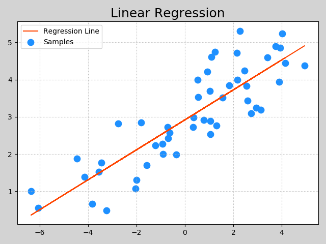
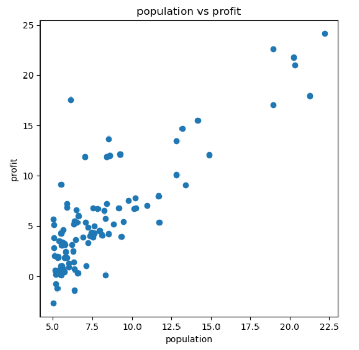
吳恩達機器學習課程-作業1-線性回歸(python實現) 椰汁學習筆記 最近剛學習完吳恩達機器學習的課程,現在開始復習和整理一下課程筆記和作業,我將陸續更新。 Linear regression with one variable 2.1 Plotting the Data 首先我們讀入數據,先觀察數據的內容 數據是一個txt文件,每一行存儲一組數據,第一列數據為城市的人口,第二列數據城市飯店的利...

My Machine Learn(二): 邏輯回歸(Logistic Regression)
一、簡介 老規矩,先來看看度娘她老人家是如何描述邏輯回歸的: logistic回歸又稱logistic回歸分析,是一種廣義的線性回歸分析模型,常用于數據挖掘,疾病自動診斷,經濟預測等領域 。 也就是說,你也可以把邏輯回歸看做是線性回歸的一個分支或特例, 就好像“正方形”是“矩形”的特例一樣。 我在網上也瞧了不少與邏輯回歸相關的文章,基本上一上來就是一...
Machine Learning in Action 5. Logistic Regression
1. Logistic Regression 解決問題: 二分類問題(binary classification) 分類器: 為了實現logistic回歸分類器,可以在每個特征上都乘以一個回歸系數(權重),把所有結果值相加,總和(y= w1x1+w2x2+…+b)代入sigmoid函數中,從而得到一個范圍在0-1之間的數值。任何大于0.5的數被分入1類,小于0.5被分入0類。 所以l...
猜你喜歡
Machine Learning(regression)
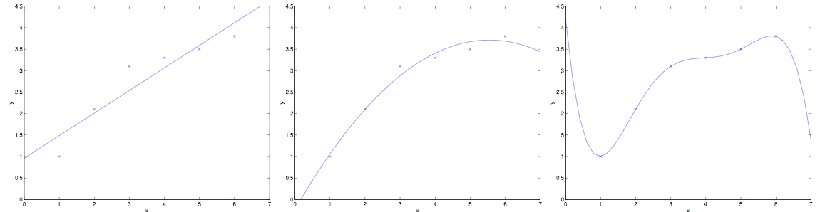
Machine Learning 回歸問題 一.LinearRegression 二.Ridge(嶺回歸) 三.polyfit(多項式回歸) 四.AdaBoost決策樹與AdaBoost(正向激勵) Feature Importance: 五.randomForestRegressor(隨機森林)...
Machine Learning Linear Regression
線性回歸的概念 1、線性回歸的原理 2、線性回歸損失函數、代價函數、目標函數 3、優化方法(梯度下降法、牛頓法、擬牛頓法等) 4、線性回歸的評估指標 5、sklearn參數詳解 1、線性回歸的原理 進入一家房產網,可以看到房價、面積、廳室呈現以下數據: | | | 面積($x_1$) 廳室數量($x_2)$ 價格(萬元)(y) 64 3 225 59 3 185 65 3 208 116 4 50...
Andrew Ng Machine learning——Work(One)——Linear regression——Univerate(Based on Python 3.7)
所用數據鏈接::https://pan.baidu.com/s/1YGsencu8wrilvrjuSteGZQ 提取碼:c3yy 目錄 Univerate linear regression 1.0 package 1.1 load data 1.2 visualization data 1.3 data preprocessing 1.4 define costfunction 1.5 grad...
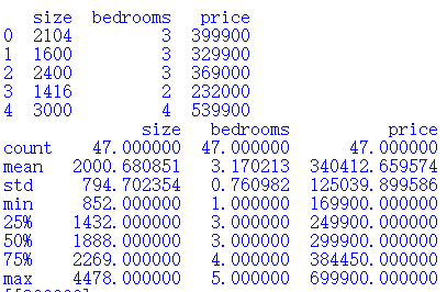
Andrew Ng Machine learning——Work(One)——Linear regression——Multivariate(Based on Pyhton 3.7)
目錄 Multivariate linear regression 1.0 package 1.1 load data 1.2 visualization data 1.3 data processing 1.4 define costfunction 1.5 gradientdescend 1.6 visualization result 1.7 prediction Multivariate ...
